On the Similarity between Hidden Layers of Pruned and Unpruned

Convolutional Neural Networks

Alessio Ansuini

, Eric Medvet

1 b

, Felice Andrea Pellegrino

1 c

and Marco Zullich

1 d

Dipartimento di Ingegneria e Architettura, Università degli Studi di Trieste, Trieste, Italy

International School for Advanced Studies, Trieste, Italy

Keywords:

Machine Learning, Pruning, Convolutional Neural Networks, Lottery Ticket Hypothesis, Canonical

Correlation Analysis, Explainable Knowledge.

Abstract:

During the last few decades, artiﬁcial neural networks (ANN) have achieved an enormous success in regres-

sion and classiﬁcation tasks. The empirical success has not been matched with an equally strong theoretical

understanding of such models, as some of their working principles (training dynamics, generalization proper-

ties, and the structure of inner representations) still remain largely unknown. It is, for example, particularly

difﬁcult to reconcile the well known fact that ANNs achieve remarkable levels of generalization also in con-

ditions of severe over-parametrization. In our work, we explore a recent network compression technique,

called Iterative Magnitude Pruning (IMP), and apply it to convolutional neural networks (CNN). The pruned

and unpruned models are compared layer-wise with Canonical Correlation Analysis (CCA). Our results show

a high similarity between layers of pruned and unpruned CNNs in the ﬁrst convolutional layers and in the

fully-connected layer, while for the intermediate convolutional layers the similarity is signiﬁcantly lower. This

suggests that, although in intermediate layers representation in pruned and unpruned networks is markedly

different, in the last part the fully-connected layers act as pivots, producing not only similar performances but

also similar representations of the data, despite the large difference in the number of parameters involved.

1 INTRODUCTION

The present paper aims at exploring and connecting

two recent works on the topic of theoretical under-

standing on artiﬁcial neural networks (ANNs) work-

ing principles.

The ﬁrst of these works (Frankle and Carbin,

2019) presents an iterative pruning technique, named

Iterative Magnitude Pruning (IMP), of the parameters

of a neural network allowing to obtain sparsity lev-

els on the parameters space up to 1% of the origi-

nal, while still matching the unpruned(complete) neu-

ral network test performance. The technique consists

in iteratively pruning a ﬁxed proportion of parame-

ters having small magnitude, rewinding the network

to initialization, and re-training only the smaller sub-

network identiﬁed by the non-pruned parameters.

The second work (Raghu et al., 2017) intro-

duces Singular Vector Canonical Correlation Analy-

https://orcid.org/0000-0002-3117-3532

https://orcid.org/0000-0001-5652-2113

https://orcid.org/0000-0002-4423-1666

https://orcid.org/0000-0002-9920-9095

sis (SVCCA), a technique based on Canonical Corre-

lation Analysis (CCA) to compare two generic real-

valued matrices sharing row dimension. SVCCA is

applied to compare ANN layers by enabling a layer

to be represented as the matrix of activations of its

neurons in response to a dataset of ﬁxed, ﬁnite size.

The application of CCA yields a vector of correla-

tions, which can be averaged to obtain a similarity

measure between layers, called Mean CCA Similar-

ity.

After training convolutional neural networks with

minimal architecture on an ensemble of problems of

incremental difﬁculty based on CIFAR10

, we con-

tinue by pruning those models using IMP for a de-

sired number of iterations, obtaining a set of pruned

networks, one for each problem and iteration num-

ber. For each of those networks, we compare each

layer with its unprunedcounterpart using SVCCA (af-

ter evaluating the layer activations on a subset of the

original dataset). The obtained similarities are then

analyzed relative to the pruning ratio, the location of

the layer within the network, and the difﬁculty of the

https://www.cs.toronto.edu/ kriz/cifar.html

Ansuini, A., Medvet, E., Pellegrino, F. and Zullich, M.

On the Similarity between Hidden Layers of Pruned and Unpruned Convolutional Neural Networks.

DOI: 10.5220/0008960300520059

In Proceedings of the 9th International Conference on Pattern Recognition Applications and Methods (ICPRAM 2020), pages 52-59

ISBN: 978-989-758-397-1; ISSN: 2184-4313

classiﬁcation task.

The remainder of this paper is organized as fol-

lows. Section 2 describes the relevant related works.

Section 3 brieﬂy presents the two aforementioned

works giving an outline of the methodologies and the

underlying theory. Section 4 introduces the experi-

mental work, describing the problems on which our

networks have been trained, and explaining how the

tools have been applied on these models. Section 5

presents the numerical results of both the test perfor-

mance of the pruned networks, and the similarity be-

tween layers of pruned and unpruned networks, elab-

orating an interpretation of these ones; moreover, it

formulates some prompts for future work.

2 RELATED WORK

The contribution of the present paper is the follow-

ing: by combining two recent advances addressing

over-parametrization (Frankle and Carbin, 2019) and

hidden layers representation and comparison (Raghu

et al., 2017) in ANNs, we aim at providing a layer-

wise analysis of similarity in the representation of

CNNs for vision tasks. We here review previous

works that are somehow related to our aim.

2.1 Pruning Techniques for ANNs

Pruning techniques for ANNs have been proposed for

decades. Early attempts include L1 regularization on

the loss function (Goodfellow et al., 2016) in order to

induce sparsity in the parameters, or operating pool-

ing on the fully-connected layer(s) (Lin et al., 2013).

(Han et al., 2015) introduced a new technique

based pruning parameter with small magnitude, on

which IMP (Frankle and Carbin, 2019) is based upon.

More recently, a plethora of other techniques has

been proposed, like ADMM (Zhang et al., 2018),

or techniques for structured (block) pruning, sum-

marised in (Crowley et al., 2018).

Our paper focuses solely on IMP, while considera-

tions on other pruning techniques is left for the future.

2.2 Comparison of ANNs

Despite being a recent work, (Raghu et al., 2017) has

already prompted a number of researches utilizing

CCA in order to gain some knowledge on the simi-

larities between neural networks: for instance, (Wang

et al., 2018) use it to compare, layer-wise, the same

network when initialized differently, ﬁnding that “sur-

prisingly, representations learned by the same convo-

lutional layer of networks trained from different ini-

tializations are not similar [...] at least in terms of

subspace match”.

(Morcos et al., 2018) argued about weaknesses of

Mean CCA Similarity, instead proposing a new sim-

ilarity metric for layers, called Projection Weighted

Canonical Correlation Analysis.

On the other hand, other researches have intro-

duced different methodologies to achieve the compar-

ison: (Yu et al., 2018), for example, proposed a tech-

nique based upon the Riemann curvature information

of the “manifolds composed of activation vectors in

each fully-connected layer” of two deep neural net-

works. This technique is still at an early stage since

it enables comparison on fully-connected layers only,

and cannot be used for an analysis like ours.

(Kornblith et al., 2019), instead, offered some

considerations on CCA as a tool for layers compar-

ison in neural networks, arguing that it cannot “mea-

sure meaningful similarities between representations

of higher dimensions than the number of data points”,

hence proposingyet another methodology called Cen-

tered Kernel Alignment.

2.3 Pruned vs. Unpruned ANNs

To our knowledge, ours is the ﬁrst work concerning

an in-depth, layer-by-layer analysis of the similarities

for pruned ANNs.

(Frankle and Bau, 2019) delved into the mechan-

ics of IMP (and other related magnitude pruning tech-

niques) by analyzing the interpretability (computed

through the identiﬁcation of “convolutional units that

recognize particular human-interpretable concepts”)

of those networks, ﬁnding that pruning does not re-

duce it and prompting the conclusion that “parame-

ters that pruning considers to be superﬂuous for ac-

curacy are also superﬂuous for interpretability”. This

work does discuss the topic of pruned networks com-

parison, but it is rather a global analysis, not going

into the detail of the single layers. This work may be

thought of as an attempt, akin ours, to combine prun-

ing techniques with other recent advances in order to

gain additional insights on what may be called “prun-

ing dynamics".

(Morcos et al., 2018), instead, use CCA to com-

pare output layers of fully-trained, dense CNNs hav-

ing different number of ﬁlters in their convolutional

layers. The authors of the cited work attempt to

corroborate the Lottery Ticket Hypothesis (see Sec-

tion 3.1), but, in doing this, they do not actually oper-

ate any pruning, neither they compare hidden layers,

focusing solely on the output representation.

On the Similarity between Hidden Layers of Pruned and Unpruned Convolutional Neural Networks

3 TOOLS

3.1 Iterative Magnitude Pruning

Iterative Magnitude Pruning (IMP) is an algorithm

ﬁrst introduced in (Frankle and Carbin, 2019) to oper-

ate pruning on the parameters of a generic ANN. The

authors start by formulating a hypothesis, called Lot-

tery Ticket Hypothesis, which claims the following:

dense, randomly-initialized, feed-forwardnet-

works contain subnetworks (“winning tick-

ets”) that—when trained in isolation—reach

test accuracy comparable to the original net-

work in a similar number of iterations

This substructure may be found via an iterative

method in which the parameters with the lowest mag-

nitude get progressively skimmed from the model un-

til a target sparsity is reached.

Denoting by ⊙ the element-by-element matrix

multiplication, and deﬁned the pruning rate as the

proportion p ∈ [0, 1] of parameters we want to prune

from the network, the algorithm is the following:

Algorithm 1: IMP.

1: Randomly initialize parameters in neural net-

work, store them in structure Θ

;

2: Create trivial pruning mask M with same struc-

ture as Θ

, initialize it at 1;

3: Train the network for T iterations, store the pa-

rameters in Θ

;

4: Obtain the parameters of Θ

whose magnitude

falls below the p-th percentile; set the corre-

sponding mask entries to 0;

5: Apply the mask to the initial parameters Θ

, ob-

taining a new initialization: Θ

(1)

= Θ

⊙ M;

6: Re-train the network for other T iterations, ob-

taining a new ﬁnal conﬁguration Θ

(1)

;

7: Repeat 3–6, each time pruning only parameters

having a corresponding entry of 1 in the previous

mask, until a target sparsity rate is reached, or

performance falls below a desired threshold.

The authors showed that this algorithm effectively

ﬁnds winning tickets for shallow fully-connected and

CNNs, but fails to do so on deeper architectures, such

as VGG-19 (Simonyan and Zisserman, 2014) and

ResNet 18 (He et al., 2016), unless a warm-up phase

is employed. (Frankle et al., 2019) showed that, by

rewinding to an early-training stage of the unpruned

network (instead of rewinding at initialization), the al-

gorithm enjoys a stabler parameters conﬁguration and

is able to converge to a solution whose performance

is similar to (or better than) the complete neural net-

work.

The method for determining the mask in IMP is

referred to in (Zhou et al., 2019) as LF-Mask (Large-

Final Mask). They produced a plethora of experi-

ments using a different number of masks and rewind-

ing policies (i.e., the scalar at which each parameter

having a value of 0 within the mask gets rewound to)

showing that, generally, the LF-Mask performs better

than all of their other proposals.

3.2 SVCCA

SVCCA is a technique introduced in (Raghu et al.,

2017), and later reﬁned in (Morcos et al., 2018),

which enables the comparison between two matrices

sharing row size.

It can be applied to two generic layers of a fully-

connected neural network when they are represented

as the response of their neurons to the same ﬁxed-

size dataset. Taking a layer L

of m

neurons, L

of m

neurons, by feeding n distinct datapoints to

their respective neural networks, we may store the

neurons’ response for each of those datapoints in

matrices: L

will be represented by an n × m

ma-

trix, L

by an n × m

matrix. The authors propose

to compare those two representations using Canon-

ical Correlation Analysis (CCA), which ﬁnds two

linear transforms W

∈ R

× ˜m

, W

∈ R

× ˜m

, where

˜m = min(m

, m

), which, applied to L

, L

, yield two

sets of ˜m unit vectors Z

, Z

= L

(1)

= L

(2)

The two transformations W

, W

are determined such

that the components of Z

, Z

are pairwise orthogonal

and maximize the residual mutual Pearson correla-

tion. This correlation is called canonical correlation:

CCA hence yields ˜m values of canonical correlation:

by averaging them, a measure of similarity between

two layers is obtained, which the authors call Mean

CCA Similarity.

Moreover, it is suggested that, by operating on the

two layers a Singular Value Decomposition (SVD)

for dimensionality reduction, with the aim of keep-

ing only the singular values accounting for 99% of

the variance, one may avoid some degenerate layers

conﬁgurations which would have produced overesti-

mations in the Mean CCA Similarity. This technique

(SVD + CCA on the layers represented as matrices)

has been named Singular Vector Canonical Correla-

tion Analysis (SVCCA).

ICPRAM 2020 - 9th International Conference on Pattern Recognition Applications and Methods

Table 1: Categories composing each dataset described in

Section 4.1.

Dataset Categories

Cifar2 Automobile, Truck

Cifar4 Cifar2 + Airplane, Ship

Cifar6 Cifar4 + Cat, Dog

Cifar8 Cifar6 + Deer, Horse

Cifar10 Cifar8 + Bird, Dog

4 METHODS

As stated before, we aim at investigating, using

SVCCA, the similarities between pruned and un-

pruned layers in convolutional neural networks, the

pruned models being obtained via IMP.

For achieving this goal, we:

1. train an ensemble of convolutional neural net-

works for image classiﬁcation on subsets of the

Cifar10 dataset;

2. prune those networks using IMP;

3. compare the pruned layers with their unpruned

counterparts using CCA Mean Similarity.

All of the implementations supporting the results

described in this paper were produced on Python

3.6.4, using libraries PyTorch 1.3.0, and NumPy

1.17.2; moreover, Google’s own implementation for

SVCCA

was used.

4.1 The Problems

Cifar10 is a publicly available collection of 60000 la-

belled color images of size 32 × 32, divided into 10

classes of 6000 images each. The dataset is already

split into train (50000 images) and test (10000 im-

ages) set.

In order to increase the number of observations,

meanwhile generating correlated measurements, we

built multiple subsets over the dataset so as to obtain

a set of incrementally more difﬁcult problems. Ci-

far10 was subset over 2, 4, 6, 8 select image classes,

and the related dataset was called Cifar2, Cifar4, etc.;

the selection of classes was not operated randomly in

order not to create trivial problems, but the chosen

categories had to show, to some extent, some similar-

ities. The composition of all the categories is listed in

Table 1.

https://github.com/google/svcca

Table 2: Summary of the architectures for the CNNs for

each of the aforementioned problems. MP stands for Max-

Pooling;

indicates a layer with batch normalization;

in-

dicates a layer with dropout. Concerning training epochs T,

indicates deployment of early stopping with patience of

20 epochs and a validation dataset obtained on a stratiﬁed

random sampling of 10% of the training set observations.

Problem Conv. layers Full layers T

Cifar2 16

, 16, MP 256

, 10 50

Cifar4 16

, 16, MP, 32

32, MP

256

, 10 50

Cifar6 64

, 64, MP,

128

, 128, MP,

256

, 256, MP

256

, 10 100

Cifar8/10 64

, 64

, MP,

128

, 128

, MP,

256

, 256

, MP,

512

, 512

, MP

1024

§*

, 10 200

4.2 Convolutional Neural Networks

Architectures

The convolutional neural networks we designed were

based off of VGGNet core (Simonyan and Zisserman,

2014) Namely, the architecture consists in stacking

one or more convolutional blocks composed of 2, 3,

or 4 convolutional layers followed by a max-pooling

layer, to a fully-connected layer, eventually followed

by the output layer, having softmax activation func-

tion, and number of neurons equal to the number of

classes.

For our networks, we decided to employ batch

normalization (Ioffeand Szegedy, 2015) on some hid-

den layers (both convolutional and fully-connected)

and dropout (Srivastava et al., 2014) on fully-

connected layers only. The architectures and dataset-

speciﬁc hyperparameters are listed in Table 2.

All the networks were trained using Adam opti-

mizer (Kingma and Ba, 2014) with mini-batch size of

128, learning rate equal to 0.001, and weight decay

(L2 regularization) with parameter 0.0005. All of the

layers use the Rectiﬁed Linear Unit activation func-

tion (except for the output layer, which uses the soft-

max activation function). Moreover, for each training

mini-batch, a random data augmentation strategy was

applied consisting in a composition of cropping, hor-

izontal ﬂipping, and roto-translation.

4.3 Application of IMP

IMP was applied with a strategy similar to (Zhou

et al., 2019): we established two separate pruning

rates, p

conv

for the convolutional layers parameters,

and p

for the fully-connected layer parameters, and

On the Similarity between Hidden Layers of Pruned and Unpruned Convolutional Neural Networks

Table 3: Choices for pruning rates for the convolutional lay-

ers and fully-connected layer used during the application of

IMP.

Problem p

conv

Cifar2 0.1 0.2

Cifar4 0.1 0.2

Cifar6 0.1 0.2

Cifar8 0.2 0.2

Cifar10 0.2 0.2

operated the pruning separately for convolutional lay-

ers (pooling together all the weights and biases per-

taining to those layers and pruning the p

conv

-th pa-

rameters with the smallest magnitude) and the fully-

connected layer. The choices for pruning rates are

shown in Table 3.

After training, IMP was applied for 20 iterations.

At each iteration, the network was rewound at the

third epoch, in order to stabilize the algorithm, as in-

dicated in Section 3.1.

4.4 Layers Comparison

Since CCA, as described in Section 3.2, works on

matrices, and the convolutional layers, if represented,

as in Section 3.2, as the response of their neurons to

a given dataset, are quadridimensional tensors (data-

points × channels × vertical image size × horizontal

image size), (Raghu et al., 2017) proposed to collapse

the dimensions corresponding to the image size into

the datapoints dimension, thus reshaping the tensor in

a matrix of shape (datapoints · vertical image size ·

horizontal image size) × channels.

Once the pruned networks were obtained, we pro-

ceeded as follows. For each problem:

1. We randomly subset the (non augmented) training

dataset (problem speciﬁc) on 5000 datapoints.

2. We evaluated each network (pruned and un-

pruned) on this subset, storing the representation

of each of layer for each network. We name

= {L

(0)

, . . . , L

(K)

} the network pruned at i-th it-

eration of IMP, represented as the set of its layers,

(0)

being the input layer, L

(K)

being the output

layer; henceforth, n

represent the unpruned net-

work. Note that K is problem speciﬁc.

3. For each nework, we compared, using SVCCA,

each convolutional, pooling, or fully-connected

layer of each pruned network with its un-

pruned counterpart, i.e., L

( j)

with L

( j)

, ∀i ∈

{1, . . . , 20}, ∀ j ∈ {1, . . . , K − 1}. The similarity

was then summarized using Mean CCA Similarity

(see Section 3.2).

5 RESULTS

5.1 Test Performance

Recalling from Section 4.3, we trained 5 unpruned

convolutional neural networks on problems directly

obtained from Cifar10; each of those networks were

pruned using IMP for 20 iterations, with pruning rates

as of Table 3.

We repeated the runs of IMP 20 times, each time

starting from the same unpruned network, but using a

different seed for the optimizer.

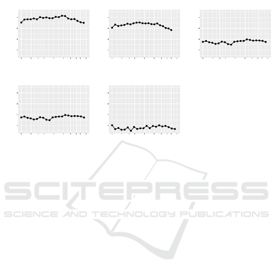
Median test accuracy of the aforementioned mod-

els, for each of iteration of IMP, are reported in Fig-

ure 1.

5.2 Layers Similarity

The results in terms of Mean CCA Similarity are

shown in Figure 2; again, since the pruning was re-

peated 20 times to increase robustness, the results,

for each layer and number of IMP iteration, are sum-

marised in the ﬁgure as median values.

We notice the presence of two different trends.

First, the neural networks for the datasets Cifar2 and

Cifar4 exhibit a decreasing similarity: (a) as the iter-

ation number increases and (b) as we progress along

the network, from input to output. If we do not con-

sider what would seem a slight incremental effect on

similarity which we can notice in almost all pooling

layers (also present in the other problems), the net-

works for Cifar2 and Cifar4 show a progressive de-

tachment from the input dataset;

Second, on the other hand, the networks for the

larger problems, Cifar6, Cifar8, and Cifar10, exhibit

a different behavior. The similarity starts high for the

ﬁrst convolutional layer, it decreases until it bottoms

around the 3rd convolutional block, ﬁnally it grows

again with a spike on fully-connected layer. More-

over, while before we noted an increasing dissimilar-

ity w.r.t. the unpruned network layers as the IMP iter-

ation increased, now the range of similarity, layer per

layer, is much smaller.

These observations, especially on the second

group of problems indicated in the list above, may

hint at some insights on the roles of the hidden layers

in convolutional neural networks as the network gets

pruned.

First of all, from all of the graphs in Figure 2, we

can notice how pruning, even at small rates, produces

layers representation which are different from the un-

pruned network ones. All the graphs seem to exhibit

trends, which, especially considering that they’re the

result of multiple trials, allow us to rule out the pos-

ICPRAM 2020 - 9th International Conference on Pattern Recognition Applications and Methods

0.86

0.88

0.90

0.92

1.000

0.500

0.300

0.200

0.100

0.050

0.030

0.020

0.015

0.010

Parameters sparsity

Test Accuracy

Cifar2

0.86

0.88

0.90

0.92

1.000

0.500

0.300

0.200

0.100

0.050

0.030

0.020

0.015

0.010

Parameters sparsity

Test Accuracy

Cifar4

0.86

0.88

0.90

0.92

1.000

0.500

0.300

0.200

0.100

0.050

0.030

0.020

0.015

0.010

Parameters sparsity

Test Accuracy

Cifar6

0.86

0.88

0.90

0.92

1.000

0.500

0.300

0.200

0.100

0.050

0.030

0.020

0.015

0.010

Parameters sparsity

Test Accuracy

Cifar8

0.86

0.88

0.90

0.92

1.000

0.500

0.300

0.200

0.100

0.050

0.030

0.020

0.015

0.010

Parameters sparsity

Test Accuracy

Cifar10

Figure 1: Median test accuracy for the models from Section 4.3. The point corresponding to Parameters sparsity equal to

1.000 refers to the unpruned model.

sibility of the results being purely the product of ran-

domness in the path of the optimizers.

Moreover, we can notice that, in harder problems,

pruning (with IMP) seems to have a stronger effect

on the convolutional layers, forcing them to produce

different representations; as we get closer to the fully-

connected layer, the network seems to be forced to

lead the representations produced by the intermediate

convolutional blocks towards a common representa-

tion for the fully-connected layer, in order to produce

a similar output, and thus getting a comparable, if not

better, test accuracy. Summarising, it would seem that

the fully-connected layer acts as a pivot during the

pruning, allowing for the network to produce simi-

lar performance despite different representations be-

ing learnt in the previous layers.

5.3 Limitations and Future Works

We remark that, as highlighted in Section 2, we are

aware of the existence of other metrics and method-

ologies for networks comparison, and we are aware

of the potential limitations of CCA raised by (Korn-

blith et al., 2019) as well. Our next step will be hence

devoted towards the incorporation of these works into

our research.

Since our work was carried out purely on a set

of convolutional neural networks for category-level

recognition, based on VGG, and trained on Cifar10,

a future goal would be to extend the analysis to other,

deeper networks (like VGG19, or Resnet 18), or to

other, more difﬁcult problems—like ImageNet (Deng

et al., 2009)—to inspect whether the same results are

observable in these networks.

Moreover, as noted by (Han et al., 2015), since

the effectiveness of pruning techniques is essentially

a consequence of the over-parameterization of ANNs,

the present work may be potentially linked to other

papers addressing the issue of over-parameterization.

For example, in (Ansuini et al., 2019), the intrinsic di-

mensionality (ID) of a layer in a deep neural network

(i.e., the “minimal number of coordinates which are

necessary to describe its points without signiﬁcant in-

formation loss”) is analyzed. The authors computed

the ID of layers for an ensemble of convolutional neu-

ral networks for image classiﬁcation observing that

the ID was exhibiting a bell-shaped trend, somewhat

complementary to what we observed in our research

in Figure 2 for the three largest models: the ID started

low, increased, spiked at around 30–40% of the net-

work depth, then decreased, bottoming at the output

layer. A direction of future work is studying whether

the shape for layer-wise similarity in our research may

somewhat be connected to these observations on ID,

i.e., that the decrease in similarity in the mid-ranked

convolutional layers is low because ID of these lay-

ers is high, and, on the other hand, a low ID in the

early and later layers is what causes the representa-

tions to be similar as far as Mean CCA Similarity is

concerned.

On the Similarity between Hidden Layers of Pruned and Unpruned Convolutional Neural Networks

0.4

0.5

0.6

0.7

0.8

0.9

1.0

conv

pool

f−c

Layer

Mean CCA similarity

Ite

Cifar2

0.4

0.5

0.6

0.7

0.8

0.9

1.0

conv

pool

conv

pool

f−c

Layer

Mean CCA similarity

Ite

Cifar4

0.4

0.5

0.6

0.7

0.8

0.9

1.0

conv

pool

conv

pool

conv

pool

f−c

Layer

Mean CCA similarity

Ite

Cifar6

0.4

0.5

0.6

0.7

0.8

0.9

1.0

conv

pool

conv

pool

conv

pool

conv

pool

f−c

Layer

Mean CCA similarity

Ite

Cifar8

0.4

0.5

0.6

0.7

0.8

0.9

1.0

conv

pool

conv

pool

conv

pool

conv

pool

f−c

Layer

Mean CCA similarity

Ite

Cifar10

Figure 2: Median values of Mean CCA Similarity between pruned layers and their unpruned counterparts for models, and

IMP iteration number, from Section 4.4. Layers are ordered, left to right, from closer to input to closer to output. Line color

shade is related to iteration number of IMP.

6 CONCLUSIONS

In this paper, we applied IMP to CNNs based on

VGG, trained on an set of increasingly difﬁcult prob-

lems derived from Cifar10. We then inspected the

layer-wise similarities between unpruned and pruned

networks using SVCCA. For the more difﬁcult prob-

lems, as we got farther from the input layer, we ob-

served a decreasing similarity, bottoming at around

half of the network depth, and then an increase, as

the fully-connected layer is approached. That behav-

ior may indicate that the fully connected layer plays a

role of pivot for leading the differences produced by

convolutional layers back to somewhat similar repre-

sentations.

Future work includes exploiting some very recent

advances in the similarity measures for network lay-

ers and exploring the connection to existing results

on the over-parameterization in artiﬁcial neural net-

works.

REFERENCES

Ansuini et al., 2019Ansuini, A., Laio, A., Macke, J. H., and

Zoccolan, D. (2019). Intrinsic dimension of data rep-

resentations in deep neural networks. In NIPS 2019.

Crowley et al., 2018Crowley, E. J., Turner, J., Storkey, A.,

and O’Boyle, M. (2018). Pruning neural networks:

is it time to nip it in the bud? arXiv preprint

arXiv:1810.04622.

Deng et al., 2009Deng, J., Dong, W., Socher, R., Li, L.-J., Li,

K., and Fei-Fei, L. (2009). ImageNet: A Large-Scale

Hierarchical Image Database. In CVPR09.

Frankle and Bau, 2019Frankle, J. and Bau, D. (2019). Dis-

secting pruned neural networks. arXiv preprint

arXiv:1907.00262.

Frankle and Carbin, 2019Frankle, J. and Carbin, M. (2019).

The lottery ticket hypothesis: Finding sparse, train-

able neural networks. In International Conference on

Learning Representations.

Frankle et al., 2019Frankle, J., Dziugaite, G. K., Roy, D. M.,

and Carbin, M. (2019). Stabilizing the lottery ticket

hypothesis. arXiv preprint arXiv:1903.01611.

Goodfellow et al., 2016Goodfellow, I., Bengio, Y., and

Courville, A. (2016). Deep learning, chapter 7.1.2 -

L1 Regularization. MIT press.

Han et al., 2015Han, S., Pool, J., Tran, J., and Dally, W.

(2015). Learning both weights and connections for ef-

ﬁcient neural network. In Cortes, C., Lawrence, N. D.,

Lee, D. D., Sugiyama, M., and Garnett, R., editors,

Advances in Neural Information Processing Systems

28, pages 1135–1143. Curran Associates, Inc.

He et al., 2016He, K., Zhang, X., Ren, S., and Sun, J. (2016).

Deep residual learning for image recognition. In Pro-

ceedings of the IEEE conference on computer vision

and pattern recognition, pages 770–778.

Ioffe and Szegedy, 2015Ioffe, S. and Szegedy, C. (2015).

Batch normalization: Accelerating deep network

ICPRAM 2020 - 9th International Conference on Pattern Recognition Applications and Methods

training by reducing internal covariate shift. In ICML,

pages 448–456.

Kingma and Ba, 2014Kingma, D. P. and Ba, J. (2014). Adam:

A method for stochastic optimization. arXiv preprint

arXiv:1412.6980.

Kornblith et al., 2019Kornblith, S., Norouzi, M., Lee, H., and

Hinton, G. E. (2019). Similarity of neural network

representations revisited. In ICML, pages 3519–3529.

Lin et al., 2013Lin, M., Chen, Q., and Yan, S. (2013). Network

in network. arXiv preprint arXiv:1312.4400.

Morcos et al., 2018Morcos, A., Raghu, M., and Bengio, S.

(2018). Insights on representational similarity in neu-

ral networks with canonical correlation. In Ben-

gio, S., Wallach, H., Larochelle, H., Grauman, K.,

Cesa-Bianchi, N., and Garnett, R., editors, Advances

in Neural Information Processing Systems 31, pages

5732–5741. Curran Associates, Inc.

Raghu et al., 2017Raghu, M., Gilmer, J., Yosinski, J., and

Sohl-Dickstein, J. (2017). Svcca: Singular vector

canonical correlation analysis for deep learning dy-

namics and interpretability. In Guyon, I., Luxburg,

U. V., Bengio, S., Wallach, H., Fergus, R., Vish-

wanathan, S., and Garnett, R., editors, Advances

in Neural Information Processing Systems 30, pages

6076–6085. Curran Associates, Inc.

Simonyan and Zisserman, 2014Simonyan, K. and Zisserman,

A. (2014). Very deep convolutional networks

for large-scale image recognition. arXiv preprint

arXiv:1409.1556.

Srivastava et al., 2014Srivastava, N., Hinton, G., Krizhevsky,

A., Sutskever, I., and Salakhutdinov, R. (2014).

Dropout: a simple way to prevent neural networks

from overﬁtting. The journal of machine learning re-

search, 15(1):1929–1958.

Wang et al., 2018Wang, L., Hu, L., Gu, J., Hu, Z., Wu, Y.,

He, K., and Hopcroft, J. (2018). Towards understand-

ing learning representations: To what extent do differ-

ent neural networks learn the same representation. In

Bengio, S., Wallach, H., Larochelle, H., Grauman, K.,

Cesa-Bianchi, N., and Garnett, R., editors, Advances

in Neural Information Processing Systems 31, pages

9584–9593. Curran Associates, Inc.

Yu et al., 2018Yu, T., Long, H., and Hopcroft, J. E. (2018).

Curvature-based comparison of two neural networks.

In 2018 24th International Conference on Pattern

Recognition (ICPR), pages 441–447. IEEE.

Zhang et al., 2018Zhang, T., Ye, S., Zhang, K., Tang, J., Wen,

W., Fardad, M., and Wang, Y. (2018). A systematic

dnn weight pruning framework using alternating di-

rection method of multipliers. In Proceedings of the

European Conference on Computer Vision (ECCV),

pages 184–199.

Zhou et al., 2019Zhou, H., Lan, J., Liu, R., and Yosinski, J.

(2019). Deconstructing lottery tickets: Zeros, signs,

and the supermask. arXiv preprint arXiv:1905.01067.

On the Similarity between Hidden Layers of Pruned and Unpruned Convolutional Neural Networks