
Temporally Coherent Topological Landscapes
for Time-varying Scalar Fields
Maria Herick, Vladimir Molchanov and Lars Linsen
Department of Mathematics and Computer Science,
Westf
¨
alische Wilhelms-Universit
¨
at M
¨
unster,
Einsteinstr. 62, 48149 M
¨
unster, Germany
Keywords:
Topological Landscapes, Time-varying Scalar Field Visualization.
Abstract:
Topological structures capture the main features of scalar fields. Topological landscapes have been proposed
for an intuitive depiction of n-dimensional scalar field topology using 2D landscapes with matching topology.
For time-varying scalar fields, each time step could be visualized by a 2D landscape, but there would be
no temporal coherence among the landscapes. We propose the concept of a time-varying contour tree that
is obtained by merging contour trees of all time steps into a meta data structure. The time-varying contour
tree can be exploited to generate temporally coherent topological landscapes. Visual analysis of time-varying
scalar field topology is, then, supported by animating landscapes over time or by volume rendering a stack of
temporal slices that represent color-coded landscapes.
1 INTRODUCTION
Scientific visualization is commonly concerned with
the analysis of time-varying multi-dimensional fields
representing natural phenomena. Topological repre-
sentations are an effective abstraction of a field cap-
turing its fundamental structure. A popular method
to encode a scalar field’s topology is the contour
tree (Carr et al., 2003). Since their visual represen-
tation in the form of a graph may be difficult to un-
derstand for untrained users, the metaphor of topo-
logical landscapes has been proposed for a more in-
tuitive depiction (Weber et al., 2007). A topological
landscape is an algorithmically constructed 2D scalar
field that is topologically equivalent to the original
scalar field, i.e., both fields have the same contour
tree. However, when generating a topological land-
scape for each time step individually, the landscapes
of a time-varying data set would not expose matching
structures over time.
In this paper, we propose an approach to visualize
the topological changes in time-varying scalar fields
based on the generation of temporally coherent topo-
logical landscapes. We use contour trees to represent
the structure of the scalar field of each time step. The
changes in the topology result in an evolution of con-
tour trees. We identify similarities between timesteps
and merge the contour trees to create a time-varying
contour tree, i.e., a meta data structure that stores the
temporal development of the topology. Using this
data structure, one can generate a sequence of tempo-
rally coherent topological landscapes. This sequence
can then be visualized by animating the landscapes
over time or by converting each landscape into a 2D
color image, stacking these images, and using a vol-
ume rendering approach. Our main contributions are:
• Analyzing similarities between contour trees by
defining a distance metric based on the associated
scalar field.
• Defining a meta data structure that represents a
time series of matched contour trees.
• Visualizing the temporal development of the
topology via temporally coherent topological
landscapes.
2 RELATED WORK
Isosurface and direct volume rendering are the most
prominent scientific visualization methods for 3D
scalar fields. They both rely on choosing appropri-
ate settings, i.e., isovalue or transfer function selec-
tion. Different approaches such as isosurface sim-
ilarity maps (Bruckner and M
¨
oller, 2010; Fofonov
and Linsen, 2016), stochastic distributions (Pfaffel-
moser and Westermann, 2013), or isosurface statis-
tics (Scheidegger et al., 2008) can be used to support
54
Herick, M., Molchanov, V. and Linsen, L.
Temporally Coherent Topological Landscapes for Time-varying Scalar Fields.
DOI: 10.5220/0008956300540061
In Proceedings of the 15th International Joint Conference on Computer Vision, Imaging and Computer Graphics Theory and Applications (VISIGRAPP 2020) - Volume 3: IVAPP, pages 54-61
ISBN: 978-989-758-402-2; ISSN: 2184-4321
Copyright
c
2022 by SCITEPRESS – Science and Technology Publications, Lda. All rights reserved

making such choices. Topological descriptions, in-
stead, describe all features in the scalar field.
The topological structure of a scalar field can be
extracted by representing the evolution of its isosur-
faces in the form of a Reeb graph (Reeb, 1946), which
in case of a simply connected domain (Doraiswamy
and Natarajan, 2013) becomes a contour tree (Carr
et al., 2003). Tierny et al. (Tierny et al., 2018) pre-
sented the topology toolkit to calculate topological
structures like the contour tree, which we used in
our implementation to construct merge and split trees,
i.e., the two trees that are merged to form a con-
tour tree. A common visual representation of the
extracted topology is to draw the respective graph.
For example, Heine et al. (Heine et al., 2011) dis-
cussed planar visualizations of contour trees, while
Pascucci et al. (Pascucci et al., 2004) suggested 3D
visualizations of contour trees. As the graph draw-
ings of contour trees are often hard to understand, We-
ber et al. (Weber et al., 2007) proposed topological
landscapes, which visualize the topology of a mul-
tidimensional data set by constructing a height field
with an identical contour tree. They extended the con-
cept by taking into account geometrical properties of
topological features (Beketayev et al., 2012). Harvey
et al. (Harvey and Wang, 2010) presented an ensem-
ble of volume-preserving topological landscapes from
higher-dimensional scalar fields. However, all these
approaches focus on a single scalar field, while scien-
tific data sets are commonly time-varying. Of course,
one can extract the topological landscape of each time
step individually, but the location of extracted features
of consecutive time steps would not match, which ren-
ders this approach useless for visualizing topological
changes over time.
A topological approach for time-varying data was
presented by Edelsbrunner et al. (Edelsbrunner et al.,
2004) who suggested a mathematical approach to
track changes in Reeb graphs. Such space-time topo-
logical structures can be used to track and visualize
topological features over time (Bremer et al., 2010;
Weber et al., 2011). However, such a visualization fo-
cuses on the selected topological structure only. Sim-
ilarly, Sohn et al. (Sohn and Bajaj, 2006) proposed to
compute time-varying contour topology by selecting
an isovalue and visualizing the topological changes in
the corresponding isosurfaces over time. Again, this
method is restrained to a single isovalue. Oesterling
et al. (Oesterling et al., 2017) computed time-varying
merge trees and visualize their evolution over time in
a bottom-up layout. Our time-varying contour trees
follow a similar idea, but use both merge and split
trees, which allows for a direct application to topo-
logical landscape generation.
In other contexts than contour trees, there exist
approaches that try to merge trees or graphs. For
example, Lukasczyk et al. (Lukasczyk et al., 2017)
present an approach to merge tracking graphs into
a static visualization. Also, static visualizations
when generating temporal treemaps have been pre-
sented recently by K
¨
opp and Weinkauf (K
¨
opp and
Weinkauf, 2019), which extends earlier work on sta-
ble treemaps via local moves (Sondag et al., 2018),
using Voronoi treemaps (Hahn et al., 2014), or for
evolving treemaps (Scheibel. et al., 2018). The data
structure introduced by K
¨
opp and Weinkauf is related
to our data structure presented below.
3 BACKGROUND
Let f (x,t) be a time-varying d-dimensional scalar
field sampled at spatial points {p
i
∈ R
d
|i = 1, . . . , n}
and time points t
j
, j = 1, . . . , k , i.e., the given field
values are f (p
i
,t
j
) = x
i j
. We assume that f (x, t) is a
Morse function at any time to exclude the existence of
degenerate critical points (Milnor, 2016) and that it is
defined on a simply connected set. Then, the contour
tree describes the development of isocontours in f . At
any time t
j
, the level set L
z
for an isovalue z ∈ R is de-
fined as the set of all points x ∈ R
d
with f (x, t
j
) = z.
An isocontour for isovalue z at time t
j
is then defined
as a simply connected component of L
z
.
Let T
t
j
be the contour tree of f (x, t
j
) for a fixed
time. T
t
j
is constructed by contracting each isocon-
tour for a specific isovalue of f (x,t
j
) into a point in
R
2
, which is then placed at the height indicated by
the isovalue. Thus, the edges of the contour tree rep-
resent the life span of topological features, while its
nodes symbolize critical points in the function. Crit-
ical points are points where a new isocontour occurs
(minima in f ), an existing isocontour vanishes (max-
ima in f ), multiple existing isocontours merge (saddle
points in f , referred to as merge nodes), or an exist-
ing isocontour splits (saddle points in f , referred to
as split nodes). To generate a contour tree, an inter-
mediate step is to compute a merge tree (or join tree)
and a split tree, which are directed trees that contain
only merge nodes or split nodes, respectively (Carr
et al., 2003). Subsequently, merge and split tree are
combined to form the contour tree.
As contour trees can be rather complex and their
depiction in the form of graph drawings hard to in-
terpret, Weber et al. (Weber et al., 2007) proposed to
visualize them using the metaphor of a topological
landscape, which is a 2D heightfield with a contour
tree that is identical to the contour tree of f . The
location of peaks and valleys and their area covered
Temporally Coherent Topological Landscapes for Time-varying Scalar Fields
55

provide a degree of freedom that can be used to en-
code further properties of f such as having the area
represent the volume of the topological feature.
4 TEMPORALLY COHERENT
TOPOLOGICAL LANDSCAPES
Our goal is to visualize topological changes in time-
varying scalar fields via temporally coherent topolog-
ical landscapes. Our approach starts off by comput-
ing merge and split trees for each of the given time
steps individually. We combine the merge and split
trees separately by iteratively matching the nodes of
the trees from consecutive time steps. The matching
of the nodes is based on a proper distance metric us-
ing the spatial information associated with the nodes
(Section 4.1). The aggregated merge and split trees
are combined to create the time-varying contour tree,
a meta data structure that embeds the matched con-
tour trees of all time steps (Section 4.2). The time-
varying contour tree can be used to lay out temporally
coherent topological landscapes and to visualize their
temporal development (Section 4.3).
4.1 Distance Metrics
To identify matching nodes in two (either merge or
split) trees, we recursively define a distance met-
ric for two nodes of different trees. First, we de-
fine distances between two leaf nodes. Leaves cor-
respond to isolated critical points (minima or max-
ima). Critical points are considered similar, if they
have a similar spatial location and a similar function
value. Hence, we define the distance of two leaves
i and j as the weighted sum of the Euclidean dis-
tance of the spatial locations of the respective criti-
cal points kp
i
− p
j
k
2
and the difference in their func-
tion values | f (p
i
) − f (p
j
)| (after normalizing the two
terms). Next, we define distances of two inner nodes.
Each inner node i corresponds to a connected com-
ponent R
i
in the scalar field’s domain surrounding
the point p
i
associated with the inner node. This re-
gion R
i
contains all spatial points connected to p
i
that
have a function value lower than the value assigned
to p
i
’s parent. Two inner nodes are considered sim-
ilar, if their regions match in size and location and
if the leaves of the subtrees rooted at the inner nodes
have many matches. To compute how well the regions
match, we first calculate a one-sided distance of i to a
node j by
δ
0
(i, j) =
∑
p∈R
i
\R
j
min
q∈R
j
kp − qk
2
|R
i
|
,
where | · | denotes the cardinality and k.k
2
the Eu-
clidean distance. Computations are sped up by only
considering the margins of the regions. Then, a two-
sided distance of inner nodes is defined by
δ(i, j) =
δ
0
(i, j) · |R
i
| + δ
0
( j, i) · |R
j
|
|R
i
∪ R
j
|
.
To compute how well the leaves of the subtrees match,
the average similarity of all possible leaf node pairs is
calculated as well as the percentage of matched leaf
nodes in the subtrees (if the two inner nodes were
matched). The distance measures are combined in a
weighted fashion to define the overall distance mea-
sure for inner nodes, where the weights can be ad-
justed to give one or the other aspect more impact.
We do not need to define distances for the root nodes,
as the root nodes match by definition.
4.2 Time-varying Contour Tree
Combining Two Trees. Let T
t
1
and T
t
2
with t
1
< t
2
be (either merge or split) trees, which we want to
combine to a meta tree T . Two nodes a
1
∈ T
t
1
and
a
2
∈ T
t
2
match, if they correspond to a topological fea-
ture existing in both time steps. If we detect a match,
a
1
and a
2
are combined in a single node a ∈ T . If
b
1
∈ T
t
1
or b
2
∈ T
t
2
have no match, they correspond to
a disappearing (b
1
) or appearing (b
2
) topological fea-
ture and should persist in T . Every node in T stores
information about its life span in temporal dimension
and its function values within the life span.
The algorithm for combining trees T
t
1
and T
t
2
to T
traverses the trees T
t
1
and T
t
2
top-down to build tree T
step by step. We start by matching the root nodes of
T
t
1
and T
t
2
and generating the respective root node in
T . Then, we iteratively proceed to the next depth level
of nodes in both trees. We use a greedy algorithm to
calculate the nodes’ best matching using the metrics
in Section 4.1. To find the best match for a node of
T
t
1
, we take into account that the best match may not
be at the same depth level in T
t
2
. Thus, for each node
of T
t
1
we consider the nodes of T
t
2
at the current and
the subsequent depth level and vice versa. The neces-
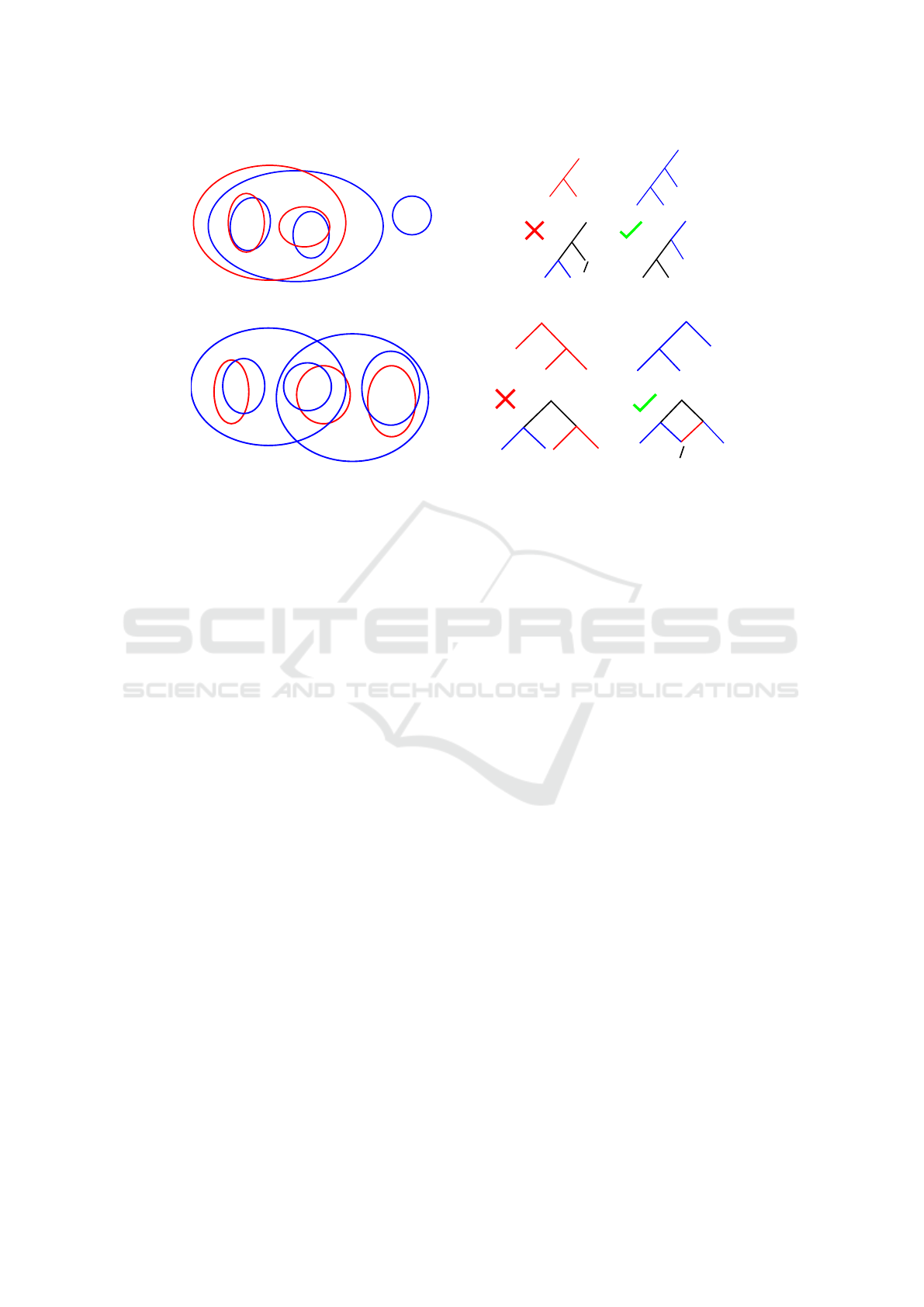
sity of taking into account the subsequent depth level
is illustrated with examples of topological changes in
Figure 1. Assuming that T
t
1
is shown in red and T
t
2
in blue, the case of an emerging topological feature
(isocontour 4) is shown in Figure 1a. Figure 1b illus-
trates that the correct match is found by shifting the
red subtree one depth level down. Figure 1c shows a
second example, where the hierarchical order of topo-
logical features changes, i.e., red isocontour 0 is a par-
ent of red isocontours 2 and 3, while blue isocontour
0 is a parent of blue isocontours 1 and 2. A correct
IVAPP 2020 - 11th International Conference on Information Visualization Theory and Applications
56

combination of T
t
1
and T
t
2
needs to have two parent
nodes of isocontour 2 in tree T , see Figure 1d. This
case destroys the tree property of T , which we have to
handle appropriately in subsequent steps. For match-
ing nodes of two trees we only consider nodes of the
current and subsequent depth level. Due to temporal
coherence, we can assume trees of consecutive time
steps to be similar to each other. Thus, we do not
proceed to further levels, which prevents exploding
computational costs.
Combining Tree Sequences. The combination of
multiple trees to one meta tree processes the trees it-
eratively in chronological order. Thus, we start by
combining T
1
and T
2
to a meta tree, then the result is
combined with T
3
, etc. Combining a tree with a meta
tree requires further considerations: As we have seen
in Figure 1, there are nodes and edges that only ex-
ist in some of the combined trees. Thus, we have to
decide which nodes and edges are to be considered
valid for the matching step. Because of temporal co-
herence of subsequent time steps, we can assume that,
e.g., T
3
is closer to T
2
than to T
1
. Hence, when adding
a tree to the meta tree of preceding time steps, only
the nodes and edges of the last time step within the
meta tree are considered during the matching, e.g., T
3
would be matched with T
2
while neglecting T
1
. This is
necessary, because the algorithm we used to calculate
the combination of the two structures relies on them
being trees. We thus need to ensure this property by
temporarily ignoring all edges that destroy it, namely
those which were described in Figure 1d. Of course,
all already existing nodes and edges in the meta tree
persist during the extension.
Generating Contour Tree. Given a sequence of
time steps, we combine the respective sequence of
merge trees and split trees separately as described
above. Then, we can join the combined merge tree
and the combined split tree to a time-varying contour
tree using the original algorithm (Carr et al., 2003).
However, this algorithm requires that merge and split
trees are actual trees, which we violated when com-
bining them, cf. Figure 1d. The requirement can be
met by duplicating the subtree whose root has two
parents (node 2 in Figure 1d). We perform such du-
plications where necessary and store a respective link
between the duplicates. Note that at any time point at
most one of the duplicates is active. Having created
the duplicates, the combined merge and split trees can
be joined using the original algorithm. The result-
ing time-varying contour tree stores all nodes of the
merge and split trees of all time steps, the respective
contour tree edges, the life span for each node and
edge, the function values of the nodes during their life
span, and links between duplicates.
4.3 Visualizing Time-varying
Landscapes
Having created the time-varying contour tree, we can
generate the topological landscape of all time steps
together using the original algorithm (Weber et al.,
2007). Of course, it is not meaningful to visualize
this landscape. Instead, we can generate topologi-
cal landscapes for each time step individually. These
landscapes are temporally coherent, as they follow the
same layout.
We can visualize the topological changes by ani-
mating the landscapes over time. For each time step,
we have stored the nodes’ height (i.e., the respective
function values), which we interpolate linearly be-
tween consecutive time steps. The animation leads to
smoothly changing renderings. The only discontinu-
ity occurs when switching between duplicates, as du-
plicates are positions at different locations in the land-
scape. However, duplicates occur at time steps when
there are topological changes. Hence, having these
steps emphasized by quickly disappearing/emerging
structures is arguably a desired effect. We color-code
duplicates in the same color to visualize the matching
structures.
Animations are suitable to show topological
changes of consecutive time steps, i.e., for temporally
local analyses. For temporally global analyses, ani-
mations induce a high cognitive load. Thus, we also
propose an alternative visualization for global analy-
ses. We transform each topological landscape into a
2D image, where for each pixel we store the heights
of the landscape and a node ID for each node of the
time-varying contour tree. We stack the 2D images in
chronological order to form a 3D image. This 3D im-
age can be rendered using a direct volume rendering
approach. By providing the node ID, we can assign to
each node a unique color in all time steps it exists. For
example, we can color-code all peaks of the topolog-
ical landscape using a categorical color map (similar
to (Weber et al., 2007)). Then, the transfer function
of the height values only maps to opacities without
changing the colors. The transfer function can be in-
teractively adjusted, e.g., to show all peaks or only
highest peaks.
5 RESULTS
To validate our approach we generated a synthetic
time-varying 2D scalar field (resolution 64 × 64, 20
Temporally Coherent Topological Landscapes for Time-varying Scalar Fields
57
1
1
2
3
2
3
4
(a)
4
32
-1
0
1
4
-1
-1
0
1
2
3
4
1
2
0
3
0
1
2 3
32
1
0
(b)
0
1
2 3
3
2
1
0
(c)
0
1 2
3
1 2
32
1
0
0
1
2 3
2
3
1
2
0
3
(d)
Figure 1: Examples for combining tree T
t
1
(red) and tree T
t
2
(blue) with occurring topological changes: Emerging isocontour
4 (a) requires us to shift to next depth level for subtree matching (b). Changing hierarchical order of isocontour 2 (c) requires
us to store two parents for the respective node in the combined tree (d).
time steps). Initially, it has two maxima, of which
one persists over time, while the other vanishes af-
ter some time steps and a third maximum emerges.
The volume rendering of the stacked topological land-
scapes in Figure 2 (left) correctly visualizes this be-
havior, where the Z-axis represents time: The per-
sisting (red), vanishing (yellow), and emerging (blue)
maxima can be easily observed. The larger areas of
the yellow and blue maxima when compared to the
red one indicate that they correspond to larger regions
in the scalar field. The transfer function has been cho-
sen to only show high values, which is why only max-
ima show up and the yellow and blue regions have
rounded shapes. Figure 2 (right) shows two time steps
of the corresponding landscape animation, namely at
the beginning (bottom) and when the red peak has
emerged while the yellow one has vanished (top).
A second synthetic time-varying 2D scalar field
example (resolution 64×64, 20 time steps) illustrates
that the merging of topological structures are also
visualized correctly (Figure 3). Here, two maxima
(green and red) fuse after some time steps and become
one maximum (blue).
Next, we applied our approach to a more com-
plicated example: We generated two 2D scalar field
with several critical points over a grid of resolution
128 × 128. Then, we produced a time-varying data
set with 20 time steps by linearly interpolating the
scalar fields at each grid point. Figure 4 shows 5
of the time steps by displaying the interpolated 2D
scalar fields on top as a grey-scale image and the cor-
responding topological landscape below. We frame
each of the extrema in the color that was assigned to
it in the topological landscape. We can observe that
the peaks in the landscape only change their heights
from Figure 4(a) to Figure 4(b). Then, in Figure 4(c),
two new maxima arise, while in Figure 4(d), a new
minimum appears. Eventually, in Figure 4(e), some
extrema vanish. We observe that the layout of the
topological landscape is stable throughout the entire
process such that it is easy to observe the changes oc-
curring in the landscapes. The accompanying video
shows the respective animation.
We also tested our algorithm on a climate reanaly-
sis data set (Copernicus Atmosphere Monitoring Ser-
vice, 2018). The data set we used consists of a time-
varying 2D temperature scalar field for 48 hours (sam-
pled every hour). Figure 5 shows three time steps of
the topological landscape animation and the respec-
tive color-coded scalar field. We observe that the
overall structure remains quite stable over time (yel-
low peak exists in all time steps), while individual
structures (several valleys) disappear.
6 DISCUSSION
Experiments showed that all components of the pro-
posed distance metric were necessary to produce de-
sired results. Adjusting the (non-zero) weights in
the distance metric does affect the result, but did
not change the main features in the overall structure.
IVAPP 2020 - 11th International Conference on Information Visualization Theory and Applications
58
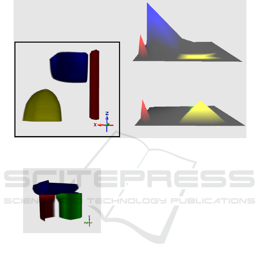
Figure 2: (left) Volume rendering of peaks for chronologically (Z-axis) stacked topological landscapes: Red peak persists
throughout the 20 time steps, while the yellow vanishes and the blue emerges. (right) Two time steps (beginning, after red
peak emerged and yellow vanished) of topological landscape animation.
Figure 3: Volume rendering of peaks for chronologically
(Z-axis) stacked topological landscapes: Two peaks (red
and green) fuse into one (blue).
Hence, the layout is stable against small changes of
the weights. The greedy approach does not guarantee
an optimal solution, but it is deterministic and pro-
duces good results. One topic for future work is to
re-consider the choice of having a discontinuity when
a topological feature switches its parent. It may be
desirable to have this discontinuity to explicitly see
such a change, but one may also argue for avoiding
it, as the feature itself is not changing but only the
parents.
Computation times were moderate for the pre-
sented examples, but optimization would be required
before applying to big data sets. For example, the
merging of time steps is currently processed sequen-
tially in chronological order. Merging consecutive
time steps in a hierarchical fashion should make the
individual computations less complex and would be
amenable to parallel computing.
7 CONCLUSION
We have presented an approach for temporally coher-
ent visualization of topological landscapes to analyze
temporally local or global topological changes. It is
based on a matching strategy of topological features
between consecutive time steps and a respective com-
bination of the contour trees. The combined contour
tree as a meta-data structure is used for the topolog-
ical landscape generation. The landscapes are then
visualized using animations of surface renderings or
using volume rendering after stacking the individual
time steps in temporal dimension. To exploit tempo-
ral coherence, we assumed that consecutive time steps
are indeed sufficiently similar.
ACKNOWLEDGEMENTS
This work was supported in part by DFG grant
MO 3050/2-1.
Temporally Coherent Topological Landscapes for Time-varying Scalar Fields
59
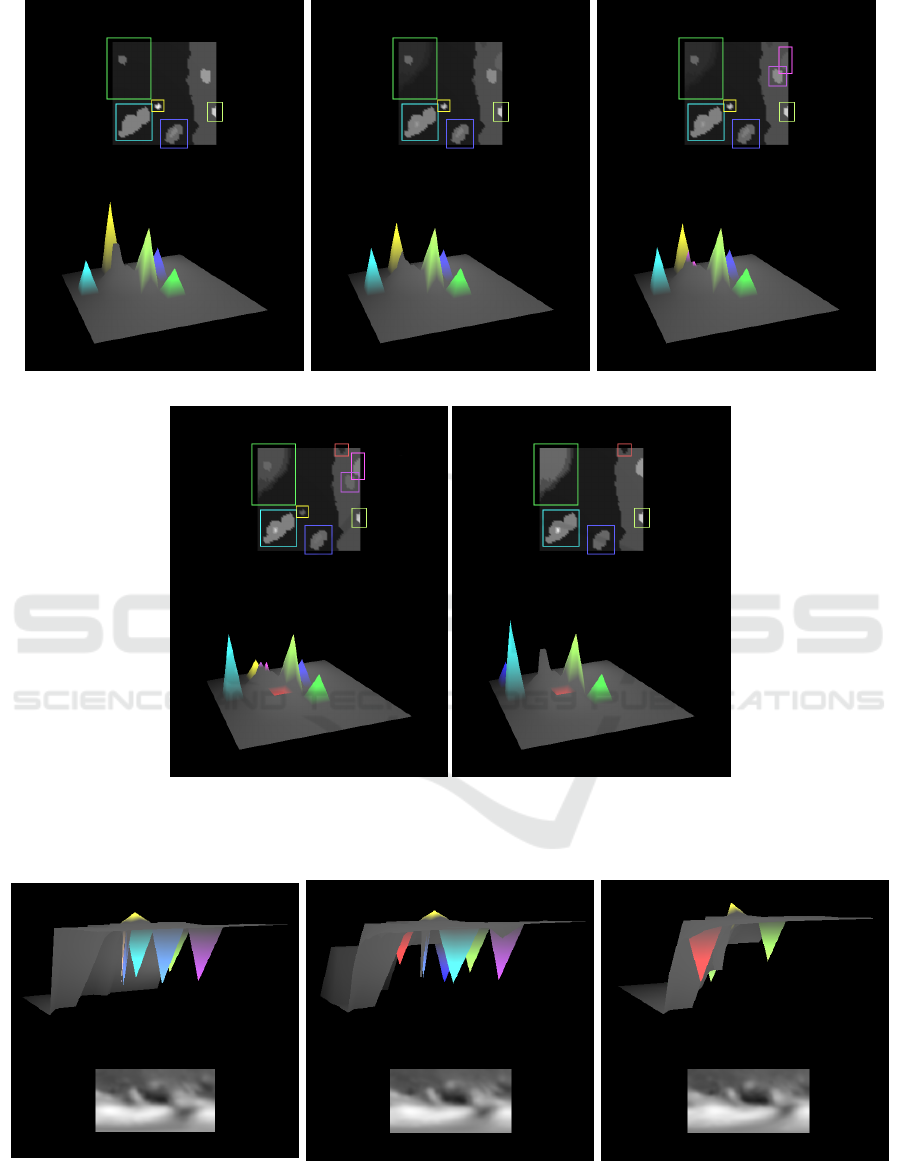
(a) (b) (c)
(d) (e)
Figure 4: Topological landscapes from a time series obtained by linearly interpolating between two 2D scalar fields with
multiple extrema. The landscapes are consistent throughout the time series such that emerging and vanishing structures as
well as height changes can be easily observed.
(a) 10 hours
(b) 20 hours (c) 34 hours
Figure 5: (top) Three time steps (after 10, 20, and 34 hours) of topological landscape animation of climate reanalysis data set.
(bottom) Color-coded visualization of respective 2D temperature fields.
IVAPP 2020 - 11th International Conference on Information Visualization Theory and Applications
60

REFERENCES
Beketayev, K., Weber, G. H., Morozov, D., Abzhanov, A.,
and Hamann, B. (2012). Geometry-preserving topo-
logical landscapes. In Proceedings of the Workshop at
SIGGRAPH Asia, WASA ’12, pages 155–160, New
York, NY, USA. ACM.
Bremer, P., Weber, G., Pascucci, V., Day, M., and Bell, J.
(2010). Analyzing and tracking burning structures in
lean premixed hydrogen flames. IEEE Transactions
on Visualization and Computer Graphics, 16(2):248–
260.
Bruckner, S. and M
¨
oller, T. (2010). Isosurface similar-
ity maps. In Computer Graphics Forum, volume 29,
pages 773–782. Wiley Online Library.
Carr, H., Snoeyink, J., and Axen, U. (2003). Computing
contour trees in all dimensions. Computational Ge-
ometry, 24(2):75–94.
Copernicus Atmosphere Monitoring Service (2018). ERA5
hourly data on pressure levels from 1979 to present.
https://cds.climate.copernicus.eu/.
Doraiswamy, H. and Natarajan, V. (2013). Computing Reeb
graphs as a union of contour trees. IEEE Transactions
on Visualization and Computer Graphics, 19(2):249–
262.
Edelsbrunner, H., Harer, J., Mascarenhas, A., and Pascucci,
V. (2004). Time-varying Reeb graphs for continuous
space-time data. In Proceedings of the twentieth an-
nual symposium on Computational geometry, pages
366–372. ACM.
Fofonov, A. and Linsen, L. (2016). Fast and robust iso-
surface similarity maps extraction using quasi-Monte
Carlo approach. In Wilhelm, A. F. and Kestler, H. A.,
editors, Analysis of Large and Complex Data, pages
497–506. Springer International Publishing.
Hahn, S., Tr
¨
umper, J., Moritz, D., and D
¨
ollner, J. (2014).
Visualization of varying hierarchies by stable layout
of voronoi treemaps. In 2014 International Confer-
ence on Information Visualization Theory and Appli-
cations (IVAPP), pages 50–58.
Harvey, W. and Wang, Y. (2010). Topological landscape
ensembles for visualization of scalar-valued functions.
In Computer Graphics Forum, volume 29, pages 993–
1002. Wiley Online Library.
Heine, C., Schneider, D., Carr, H., and Scheuermann, G.
(2011). Drawing contour trees in the plane. IEEE
Transactions on Visualization and Computer Graph-
ics, 17(11):1599–1611.
K
¨
opp, W. and Weinkauf, T. (2019). Temporal treemaps:
Static visualization of evolving trees. IEEE Transac-
tions on Visualization and Computer Graphics (Proc.
IEEE VIS), 25(1):534–543.
Lukasczyk, J., Maciejewski, R., Weber, G. H., Garth,
C., and Leitte, H. (2017). Nested tracking graphs.
Computer Graphics Forum (Special Issue, Proceed-
ings Eurographics/IEEE Symposium on Visualiza-
tion), 36(3):12–22. Best paper award.
Milnor, J. (2016). Morse Theory.(AM-51), volume 51.
Princeton university press.
Oesterling, P., Heine, C., Weber, G., Morozov, D., and
Scheuermann, G. (2017). Computing and visualizing
time-varying merge trees for high-dimensional data.
In Topological Methods in Data Analysis and Visual-
ization IV, pages 87–101.
Pascucci, V., Cole-McLaughlin, K., and Scorzelli, G.
(2004). Multi-resolution computation and presenta-
tion of contour trees. In Proc. IASTED Conference on
Visualization, Imaging, and Image Processing, pages
452–290. Citeseer.
Pfaffelmoser, T. and Westermann, R. (2013). Visualizing
contour distributions in 2D ensemble data. EuroVis-
Short Papers, 71(72):55–59.
Reeb, G. (1946). Sur les points singuliers d’une forme
de Pfaff completement integrable ou d’une fonction
numerique [on the singular points of a completely
integrable Pfaff form or of a numerical function].
Comptes Rendus Acad. Sciences Paris, 222:847–849.
Scheibel., W., Weyand., C., and D
¨
ollner., J. (2018). Evo-
cells - a treemap layout algorithm for evolving tree
data. In Proceedings of the 13th International Joint
Conference on Computer Vision, Imaging and Com-
puter Graphics Theory and Applications - Volume 3:
IVAPP,, pages 273–280. INSTICC, SciTePress.
Scheidegger, C. E., Schreiner, J. M., Duffy, B., Carr, H.,
and Silva, C. T. (2008). Revisiting histograms and iso-
surface statistics. IEEE Transactions on Visualization
and Computer Graphics, 14(6):1659–1666.
Sohn, B.-S. and Bajaj, C. (2006). Time-varying contour
topology. IEEE Transactions on Visualization and
Computer Graphics, 12(1):14–25.
Sondag, M., Speckmann, B., and Verbeek, K. (2018). Stable
treemaps via local moves. IEEE Transactions on Vi-
sualization and Computer Graphics, 24(1):729–738.
Tierny, J., Favelier, G., Levine, J. A., Gueunet, C., and
Michaux, M. (2018). The topology toolkit. IEEE
transactions on visualization and computer graphics,
24(1):832–842.
Weber, G., Bremer, P., Day, M., Bell, J., and Pascucci, V.
(2011). Feature tracking using Reeb graphs. In Topo-
logical Methods in Data Analysis and Visualization.
Mathematics and Visualization. Springer, Berlin, Hei-
delberg, pages 241–253, Berlin, Heidelberg. Springer
Berlin Heidelberg.
Weber, G., Bremer, P.-T., and Pascucci, V. (2007). Topo-
logical landscapes: A terrain metaphor for scientific
data. IEEE Transactions on Visualization and Com-
puter Graphics, 13(6):1416–1423.
Temporally Coherent Topological Landscapes for Time-varying Scalar Fields
61
