
HEp-2 Intensity Classification based on Deep Fine-tuning
Vincenzo Taormina
1 a
, Donato Cascio
2 b
, Leonardo Abbene
2 c
and Giuseppe Raso
2 d
1
Engineering Department, University of Palermo, viale delle Scienze, Palermo, Italy
2
Department of Physics and Chemistry, University of Palermo, viale delle Scienze, Palermo, Italy
Keywords: Autoimmune Diseases, IIF Test, HEp-2 Images, Deep Learning, CNN, Fine Tuning, ROC Curve.
Abstract: The classification of HEp-2 images, conducted through Indirect ImmunoFluorescence (IIF) gold standard
method, in the positive / negative classes, is the first step in the diagnosis of autoimmune diseases. Since the
test is often difficult to interpret, the research world has been looking for technological features for this
problem. In recent years the methods of deep learning have overcome the other machine learning techniques
in their effectiveness and robustness, and now they prevail in artificial intelligence studies. In this context,
CNNs have played a significant role especially in the biomedical field. In this work we analysed the
capabilities of CNN for fluorescence classification of HEp-2 images. To this end, the GoogLeNet pre-trained
network was used. The method was developed and tested using the public database A.I.D.A. For the analysis
of pre-trained network, the two strategies were used: as features extractors (coupled with SVM classifiers)
and after fine-tuning. Performance analysis was conducted in terms of ROC (Receiver Operating
Characteristic) curve. The best result obtained with the fine-tuning method showed an excellent ability to
discriminate between classes, with an area under the ROC curve (AUC) of 98.4% and an accuracy of 93%.
The classification result using the CNN as features extractor obtained 97.3% of AUC, showing a difference
in performance between the two strategies of little significance.
1 INTRODUCTION
Autoimmune diseases are particular pathologies,
which arise following a malfunction of the immune
system. In an individual with an autoimmune disease,
in fact, the cells and glycoproteins, which make up
the immune system, attack the organism which they
should instead defend against pathogens and other
threats present in the external environment.
Autoimmune diseases are increasing in the general
population, both due to an actual increase in
prevalence and to an improvement in diagnostic tools,
where the laboratory plays a fundamental role.
Autoantibody research is an integral part of both
classification and remission criteria for many
autoimmune diseases. Indirect ImmunoFluorescence
(IIF) is the most commonly used technique for the
determination of anti-nucleus antibodies due to its
sensitivity, ease of execution and low cost.
a
http://orcid.org/0000-0002-8313-2556
b
http://orcid.org/0000-0001-6522-1259
c
http://orcid.org/0000-0001-9633-6606
d
http://orcid.org/0000-0002-5660-3711
Antinuclear antibodies (ANA) represent a vast and
heterogeneous antibody population, especially of the
IgG class, directed towards different components of
the cell nucleus (DNA, ribonuclear proteins, histones,
centromere). For the execution of the IIF technique,
as a substrate, the use of epithelial cells from human
laryngeal cartilage (HEp-2) is recommended, in
which the expression and integrity of clinically
significant antigens are guaranteed. The result of the
ANAs should be interpreted as positivity or negativity
with respect to the screening dilution used.
In the past years, a great deal of effort was put into
research regarding Indirect ImmunoFluorescence
techniques with the aim of development of CAD
systems (Hobson, 2016), (Cascio, 2019).
As it is aimed at identifying the patient's
positivity/negativity to the test, the fluorescence
intensity classification phase is very important.
Moreover, as regards the CAD system, it will be the
result of this phase to establish (in the case of positive
Taormina, V., Cascio, D., Abbene, L. and Raso, G.
HEp-2 Intensity Classification based on Deep Fine-tuning.
DOI: 10.5220/0008954501430149
In Proceedings of the 13th International Joint Conference on Biomedical Engineering Systems and Technologies (BIOSTEC 2020) - Volume 2: BIOIMAGING, pages 143-149
ISBN: 978-989-758-398-8; ISSN: 2184-4305
Copyright
c
2022 by SCITEPRESS – Science and Technology Publications, Lda. All rights reserved
143
output) if the execution of the analysis steps aimed at
identifying the staining patterns present in the image
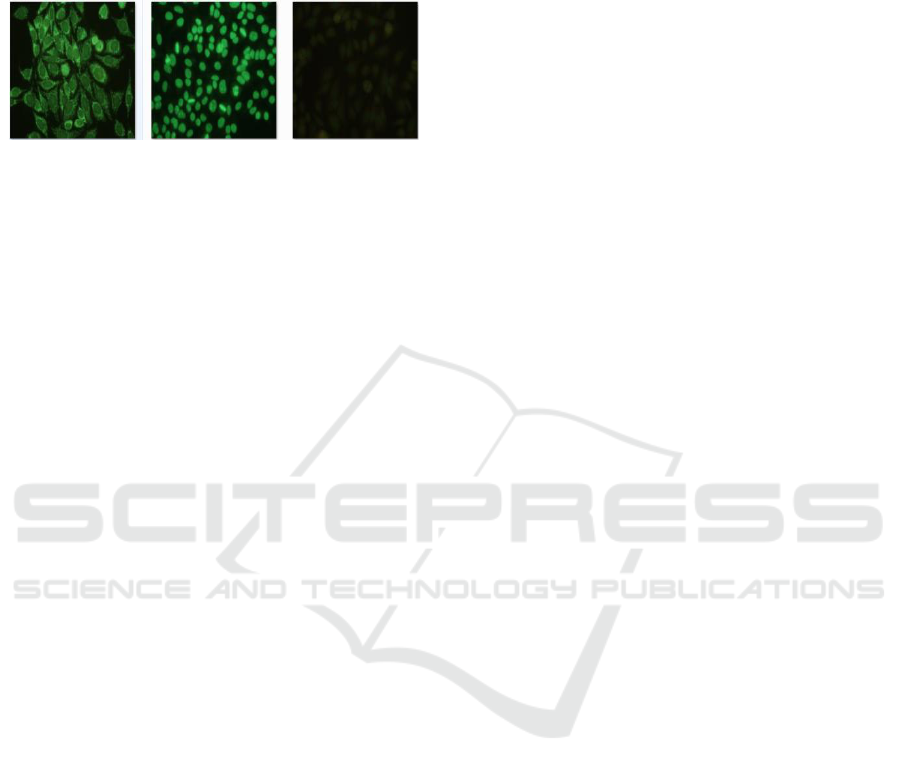
will be carried out. Figure 1 shows examples of
positive/negative class.
Figure 1: IIF images with different fluorescence intensity:
on the left is a positive cyctoplasmatic image, in the center
there is a positive nuclear image and on the right a negative
image is shown.
1.1 Related Work
Below we briefly describe the major works in the
field of HEp-2 image analysis. One of the first
significant advances in the field was proposed by
Perneret al. (Perner, 2002) presented an early attempt
on developing an automated HEp-2 cell classification
system. Cell regions were represented by a set of
basic features extracted from binary images obtained
at multiple grey level thresholds. Those features were
then classified into six categories by a decision tree
algorithm.
The problem of HEp-2 cell classification attracted
major attention among researchers with the
benchmarking contests (Foggia 2014).
The method that won the competition presided by
Manivannan et al (Manivannan, 2016) reached a
mean class accuracy equal to 87.1%. Their method
extracts a set of local features that are aggregated via
sparse coding. They use a pyramidal decomposition
of the cell analysed in the central part and in the
crown that contains the cell membrane. Linear
support vector machines (SVMs) are the classifiers
used on the learned dictionary, specifically they use 4
SVM the first one trained on the orientation of the
original images and the remaining three respectively
on the images rotated by 90/180/270 degrees.
In our previous studies (Cascio, 2016) we have
addressed the problem of pattern classification, we
proposed a classification approach based on a one-
against-one (OAO) scheme. To do this, fifteen SVM
with gaussian RBF (Radial Basic Function) kernel
have been trained.
In some papers unsupervised methods are
proposed to address the HEp-2 image classification
(Vivona, 2016), (Gao, 2014), (Vivona, 2018).
One of the first researchers to use CNN in the
classification of HEp-2 images is GAO (Gao, 2016)
The authors used a CNN with data augmentation.
Specifically, it contains eight layers. Among them,
the first six layers are convolutional layers alternated
with pooling layers, and the remaining two are fully-
connected layers for classification. They compared
the method with traditional methods such as BoF and
FV fisher vector.
Also in the work of Li et al (Li, 2016) the authors
proposed CNNs for the solution of the classification
problem. The authors proposed a method which
consists in the use of a CNN to construct a Histogram
Pattern and through this a linear SVM is trained. In
their work the authors show that the strategy that uses
SVM outperforms that of cell prevalence.
Oraibi et al (Oraibi, 2018) used the well-known
pre-trained CNN VGG-19 network to extract features
and combine them with local features such as RIC-
LBP (Rotation Invariant Cooccurence Local Binary
Pattern) and JML (Joint Motif Labels). The
combination of features was used to train RF
classifiers (random forest).
In (Cascio, 2019) CNN pre-trained Alexnet is
used as a feature extractor in combination with using
six linear SVM and a KNN classifier as a collector to
classify six pattern.
Despite the growing interest of the scientific
community, the problem of identifying the
fluorescence intensity was still little addressed.
In this context, Merone et al (Merone, 2019) use
the ScatNet network. They extract the features from
the green channel only. However, the authors do not
make a classification between positive and negative,
but between positive and weak positive.
Benammar et al (Benammar, 2016) have
optimized and tested a CAD system on HEp-2 images
able to classify the fluorescene intensity. The system
classifies positive/negative images using one SVM
classifier. Results showed 85,5% of accuracy in
intensity fluorescence detection.
Di Cataldo et al., (2016) presented a method,
ANAlyte, which is able to characterize IIF images in
terms of fluorescent intensity and fluorescent pattern.
They obtained overall accuracy of fluorescent
intensity around 85%.
In our previous work (Cascio, 2019) the problem
of fluorescence intensity classification using pre-
trained networks as feature extractors was addressed.
The method was tested using a public database. The
best configuration allowed an accuracy of 92.8%.
In this paper we describe a system for the
positive/negative intensity HEp-2 image
classification. In particular, considering the
effectiveness of CNN demonstrated in the field of
medical imaging classification, in this work we
BIOIMAGING 2020 - 7th International Conference on Bioimaging
144

decided to use and test the GoogLeNet (Szegedy,
2015) pre-trained network. A fine-tuning carried out
different training modalities has been realized. The
strategy of using CNN as a feature extractor was also
evaluated, coupled with a SVM classifier, and the
classification results were compared.
2 MATERIALS AND METHODS
2.1 Image Dataset
For this work we used a public image database HEp-
2 A.I.D.A. project (Cascio, 2019). To date, to our
knowledge, the database A.I.D.A. is the only public
database that contains both positive and negative
images. The other two main HEp-2 images public
dataset I3A (Lovell, 2014) and MIVIA
(https://mivia.unisa.it/datasets/biomedical-image-
datasets/hep2-image-datase)contains only positive
and weak positive images but not negative cases. The
public A.I.D.A. database is composed of 2080
images; 582 are negative while 1498 show a positive
fluorescence intensity. The images have 24 bits color
depth and are stored in common image file formats.
The A.I.D.A. database can be downloaded, after
registration, from the download section of the site
(http://www.aidaproject.net/downloads).
2.2 Cross-validation Strategy
The strategy used for the training-validation-test
chain was the k-fold validation considering the
specimens. In fact, since images belonging to the
same specimen are very similar, in the case in which
images of the same well were used both in the training
and in the test, the result of the classification would
be distorted (Manivannan, 2016) (Iacomi, 2014). In
this work, a k = 5 was chosen, so the DB was divided
into 5 folds. With this strategy we carry out 5
trainings and the relative tests. Approximately at each
iteration 20% of the dataset was used for the test, the
remaining 80% divided into training and validation to
the extent of approximately 64% and 16% of the
dataset. For the optimization of the parameters and for
the test the area under the ROC (Receiver Operating
Characteristic) curve (AUC) was used as merit
figures.
2.3 Convolutional Neural Network
The CNN imitates how the visual cortex of the brain
processes images. In recent years, scientific research
in the field of machine learning has shown that the
use of CNN networks has improved the efficiency of
image classification in various fields of application of
pattern recognition. The traditional chain
"preprocessing - features extraction - training model"
(derive model from training data) has been replaced
by CNNs which in their training process include
features extraction (design model - training CNN
model). Despite the first neural networks and CNNs
date back to the 80s / 90s only in recent years have
they overcome the traditional techniques, above all
thanks to the introduction of the ReLU activation
fuction, of the dropout, and thanks to the increased
computing power provided by the GPUs.
Nonetheless, their effectiveness has increased thanks
to the possibility of using Datasets of a larger size. In
general, a CNN can be represented as the composition
of two blocks (see Figure 2); the first presents
convolutional layers and pooling layers while the
second presents a deep neural network. The entry of
CNN is an image while the output is a probability in
the case of binary problems, or a vector of probability
in the case of multi-class problems.
The design and training of a CNN is an extremely
complex problem, both for the necessary data but also
for the useful computing power. One way to
overcome the problem in the literature is to use pre-
trained CNN networks. Thanks also to competition
like ImageNet, extremely performing CNN networks
have been created and published that are able to
classify images in 1000 object categories.
Pre-trained CNNs can be used considering the
following two strategies:
1) as feature extractors and coupled to a traditional
classifier such as the appropriately trained SVM;
2) performing pre-trained CNN transfer learning; in
this case, by appropriately replacing the last layer
based on the classes to be discriminated, fine-
tuning is performed using the database of data to
be classified in the training.
In this work we have analyzed both the startegies and
to do this we have used one of the most well-known
and peforming CNN network, that is GoogleNet. This
network is based on the use of "inception modules",
each of which includes different convolutional sub-
networks concatenated at the end of the module. This
network is composed of 144 layers. The inception
blocks consist of four branches, the first three with
1x1, 3x3 and 5x5 convolutions, the fourth with a 3x3
max pooling. The last layers are composed of an
average pooling and a fully connected layers and the
softmax for the final output.
HEp-2 Intensity Classification based on Deep Fine-tuning
145
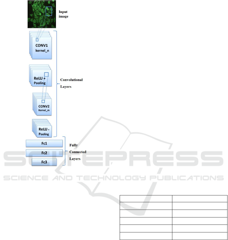
Figure 2: CNNs general scheme.
2.4 Hyperparameter Optimization
The design of a generic CNN provides, in addition to
establishing the architecture and the topology, the
optimization of parameters and connections' weights
through optimization procedures in the training
phase. We refer to the many values to be optimized as
hyperparameters optimization. Pre-trained CNNs
have a consolidated and database-optimized
architecture for which they were originally trained.
For the optimization of the parameters in the
training phase it is necessary to observe the training
algorithm optimization. The latter represents the
algorithm for updates the weights and the biass of
network. Among the most recognized methods is the
Stochastic Gradient with Momentum (SGDM) which
minimizes the loss function at each iteration
considering the gradient of the loss function on the
entire training dataset. The momentum term serves to
reduce the oscillations of the SGD algorithm along
the path of steepest descent towards the optimum. The
momentum is responsible for reducing some of the
noise and oscillations in the high curvature of the loss
function. A variant of the SGD uses subsets of the
training called mini-batchs, in this case a different
mini-batch is used at each iteration. In short, the mini-
batch specifies how many images to use at each
iteration. The full pass of the training algorithm over
the entire training set using mini-batches is one
epoch. In addition to SGDM, there are other
algorithms known as RMSProp (Root Mean Square
Propagation) and ADAM (Adaptive Moment
estimation); however in this work we have chosen to
use SGDM with mini-batch. The choice of the SGDM
was made because the stochastic gradient descent
algorithm can oscillate along the path of steepest
descent towards the optimum. Adding a momentum
term to the parameter update is one way to reduce this
oscillation (Murphy, 2012).
Another fundamental factor of the training
process is the Learning Rate: defines the level of
adjustments of weight connections and network
topology, applied at each training cycle. An small
learning rate permits a surgical fine-tune of the model
to the training data, at the cost of higher number of
training cycles and processing time. A high learning
rate permits the model to learn more quickly, but may
sacrifice its accuracy caused by the lack of precision
over the adjustments. This value is usually set in 0.01,
but in some cases it is interesting to be fine-tuned,
especially if you want to improve the runtime when
using SGD (Bengio, 2012) .
Table 1 shows the search space used for parameter
optimization in this work.
Table 1: Hyperparameters grid search.
parameter
Total layers
Training mode
SGDM with Mini-batch
Minibatch size
{4, 8, 16, 32, 64, 128}
Learning Rate
{0.01, 0.001, 0.0001}
Momentum coef.
0.9
Epoch
max 10 epoch
2.5 Training Strategy and
Classification
The fine-tuning approach for the googleNet pre-
trained network was analyzed. The parameters were
optimized by performing a training using the IIF
image database. In general, to implement fine tuning,
the last layer must be replaced to correctly define the
number of classes to be discriminated. In the present
work, since it discriminates between two classes, the
problem turns out to be binary. It is also a common
pratice to freeze the weights/parameter of the first
BIOIMAGING 2020 - 7th International Conference on Bioimaging
146
layers of the pre-trained network. The parameters /
weights of the first CNN layers are frozen and the
training on the remaining parameters / weights is
performed. This is because the first few layers capture
universal features like curves and edges that are also
relevant to our new problem. We want to keep those
weights intact. Instead, we will get the network to
focus on learning dataset-specific features in the
subsequent layers.
We used pre-trained CNN network was trained
with fine tuning by considering three different depths
of freeze. Table 2 shows the number of frezeed layers
(on the total of 144 levels) for the different tuning
levels performed.
Table 2: Analyzed freezing levels.
First
level
(soft)
Second
level
(medium)
Third level
(hard)
layers freezed
11
110
139
Moreover CNN has been evaluated as feature
extractors both in the pre-trained configuration and
after fine-tuning; as features extractor CNNs have
been coupled to linear SVM classifiers. The main
feature of the SVMs is their simplicity in terms of
parameters makes it possible to tackle complex
classification problems in which there are, as in our
case, a large number of input features. This need for
simplicity has led us to implement a SVM classifier
with linear kernel, the simplest in terms of parameters
to search. Considering the high-dimensional features
vector extracted we have chosen to use the linear
kernel (instead of non-linear others such as Gaussian
kernel) to cotain the computation. For this, we have
used the efficient Matlab ”fitclinear” (MATLAB
Release 2019a, The MathWorks, Inc., Natick,
Massachusetts, United States). Matlab’s “logspace”
function in the range between 10
-6
and 10
2.5
was used
as the parameter search method for the linear kernel;
20 equidistant values on a logarithmic scale were
analyzed.
To increase the number of training examples, a
data augmentation was made. In particular, an
increase for image rotation at angles of 20°was
achieved; overall, a multiplication of the data by a
factor of 18 was obtained. Data augmentation is a
very effective practice especially when the data set
for training is limited, or as in our case, when some
classes are not particularly represented in the set of
examples. The effect of this data augmentation was
valued quantitatively in terms of performance.
3 RESULTS
As regards the fine-tuning strategy, the best results
obtained, in terms of AUC, are reported in Table 3.
Table 3: CNN performance analysis implemented with
fine-tuning strategy.
Freeze
first level
Freeze
second
level
Freeze
third level
Freeze
firstlevel
+data augm.
AUC
98.0%
96.8%
96.3%
98.4%
The best result among the three freezing levels
analyzed was obtained from the first level. For this
configuration, training with data augmentation was
also evaluated, which showed a slight increase in
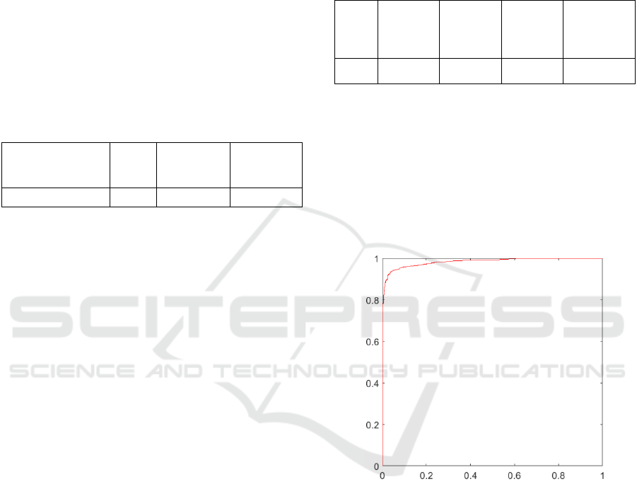
classification performance. The Hyperparameter
related to the best configuration obtained were:
Learning Rate = 0.01, Minibatch = 16, Epoch = 7.
The ROC curve obtained from this configuration
is shown in Figure 3.
Figure 3: ROC curve obtained from the best fine-tuning
configuration.
For all the training images the features have been
extracted from various layers of the GoogleNet
network and the C parameter of the SVM classifier
has been optimized for validation. The layer that
allowed the best result is the "inception_3a-output".
The parameter relative to the best performing
configuration was C = 5.1348. The best CNN
configuration used as a feature extractor achieved an
AUC = 97.3%.
The results obtained in this work were compared
with other works of the state of the art and the
comparison presented in Table 4.
From the comparison presented in the Table 4 it is
easy to infer the classification effectiveness of CNN
HEp-2 Intensity Classification based on Deep Fine-tuning
147

applied to HEp-2 images. In particular, the fine-
tuning strategy proved to be more effective of the
CNN layers features extraction strategy, both in
accuracy and in AUC, of about 1%.
Table 4: Performance comparison between intensity
classification methods on HEp-2 images.
Images
dataset
Accuracy
AUC
Di Cataldo
(Di Cataldo, 2016)
71
85.7%
-
Benammar
(Benammar, 2016)
1006
85.5%
-
Cascio
(Cascio, 2019)
2080
92.8%
97.4%
Our method
2080
93.0%
98.4%
4 CONCLUSIONS
In this paper a method for the automatic classification
of fluorescence intensity in HEp-2 images was
presented. This classification is very important for a
correct diagnosis of autoimmune diseases. A method
that uses the well-known GoogLeNet pre-trained
network has been presented. The potential of the
network has been analysed, with a view to optimizing
the classification process, with two strategies: as
feature extractors, in combination with the traditional
SVM classifier, and as classifiers after an appropriate
fine-tuning process. Different levels of freezing were
analysed and the improvement in performance of the
data augmentation was evaluated. The method, which
was developed and tested using a public database,
showed high classification performance: AUC of
98.4%. A comparison with other works of the state of
the art reveals the goodness of the proposed method
and the capabilities of GoogLeNet in the
classification of HEp-2 type images.
In the future, we planned to investigate the use of
ad-hoc CNN architectures instead of pre-trained
CNN. In addition, a study is in progress using several
pre-trained networks in order to identify the best
configuration for the HEp-2 image intensity analysis.
REFERENCES
Benammar, A., et al, 2016. Computer-assisted
classification patterns in autoimmune diagnostics: the
AIDA project.BioMed research international.
Bengio, Y., et al, 2012.Pratical Recommendations for
Gradient-Based Training of Deep Architectures.
Springer Berlin Heidelberg, pp. 437-478.
Cascio, D., et al, 2016. A multi-process system for HEp-2
cells classification based on SVM. Pattern Recogn.
Lett., 82, 56-63.
Cascio, D., et al, 2019. An Automatic HEp-2 Specimen
Analysis System Based on an Active Contours Model
and an SVM Classification.Applied Sciences, vol. 9, pp.
307.
Cascio, D., et al, 2019. Deep Convolutional Neural
Network for HEp-2 Fluorescence Intensity
Classification. Applied Sciences.
Cascio, D., et al, 2019. Deep CNN for IIF Images
Classification in Autoimmune Diagnostics.Applied
Sciences, vol. 9, pp. 1618.
Di Cataldo, S., et al, 2016. ANAlyte: A modular image
analysis tool for ANA testing with indirect
immunofluorescence. Computer methods and
programs in biomedicine, vol. 128, pp. 86-99.
Foggia, P., et al, 2014. Pattern recognition in stained HEp-
2 cells: Where are we now?.Pattern Recognition, 47,
2305-2314.
Gao, Z., et al, 2014. Experimental study of unsupervised
feature learning for HEp-2 cell images clustering.
InDICTA International Conference on Digital Image
Computing: Techniques and Applications.
Gao, Z., et al, 2016. HEp-2 cell image classification with
deep convolutional neural networks.IEEE Journal of
Biomedical and Health Informatics, vol. 21, pp. 416-
428.
Hobson, P., et al, 2016.Computer Aided Diagnosis for Anti-
NuclearAntibodies HEp-2 images: Progress and
challenges. Pattern Recognition Letters, vol. 82, pp. 3-
11.
Iacomi M., et al, 2014. Mammographic images
segmentation based on chaotic map clustering
algorithm. BMC Medical imaging, vol. 14.
Li, H., et al, 2016. HEp-2 specimen classification via deep
CNNs and pattern histogram. In ICPR 2016, 23rd
International Conference on Pattern Recognition.
Manivannan, S., et al, 2016. An automated pattern
recognition system for classifying indirect
immunofluorescence images of HEp-2 cells and
specimens. Pattern Recognition, 51, 12-26.
Merone, M., et al, 2019. A computer-aided diagnosis
system for HEp-2 fluorescence intensity
classification.Artificial intelligence in medicine, vol.
97, pp. 71-78.
Murphy, K. P., 2012. Machine Learning: A Probabilistic
Perspective. The MIT Press, Cambridge,
Massachusetts.
Oraibi, Z., et al, 2018.Learning Local and Deep Features for
Efficient Cell Image Classification Using Random
Forests. In ICIP 2018, 25th International Conference
on Image Processing.
Perner, P., et al, 2002.Mining knowledge for Hep-2 cell
image classification. Artificial Intelligence in Medicine,
26 (1-2), pp. 161-173.
BIOIMAGING 2020 - 7th International Conference on Bioimaging
148

Szegedy, C., et al, 2015. Going deeper with convolutions.
In IEEE Conference on Computer Vision and Pattern
Recognition.
Vivona, L., et al, 2018. Automated approach for indirect
immunofluorescence images classification based on
unsupervised clustering method. IET Computer Vision,
vol. 12.
Vivona, L., et al, 2016. Unsupervised clustering method for
pattern recognition in IIF images. InIEEE IPAS 2016
International Image Processing, Applications and
Systems.
HEp-2 Intensity Classification based on Deep Fine-tuning
149
