Progressive Training in Recurrent Neural Networks for Chord

Progression Modeling

Trung-Kien Vu, Teeradaj Racharak, Satoshi Tojo, Nguyen Ha Thanh and Nguyen Le Minh

School of Information Science, Japan Advanced Institute of Science and Technology, Ishikawa, Japan

Keywords:

Recurrent Neural Network, Chord Progression Modeling, Sequence Prediction, Knowledge Compilation.

Abstract:

Recurrent neural networks (RNNs) can be trained to process sequences of tokens as they show impressive

results in several sequence prediction. In general, when RNNs are trained, their goals are to maximize the

likelihood of each token in the sequence where each token could be represented as a one-hot representation.

That is, the model learns for its sequence prediction from true class labels. However, this creates a potential

drawback, i.e., the model cannot learn from the mistakes. In this work, we propose a progressive learning

strategy that can mitigate the mistakes by using domain knowledge. Our strategy gently changes the training

process from using the class labels guiding scheme to the similarity distribution of class labels instead. Our

experiments on chord progression modeling show that this training paradigm yields signiﬁcant improvements.

1 INTRODUCTION

Recurrent neural networks (RNNs) can be used to

produce sequences of tokens, given input/output

pairs. Generally, they are trained to maximize the

likelihood of each target token given the current

state of the model and the previous target token, in

which target tokens could be in one-hot representa-

tions (Bengio et al., 2015). This training process helps

the model to learn a language model over sequences

of tokens. In fact, RNNs and their variants, such as

the Long Short-Term Memory (LSTM) and Gated Re-

current Unit (GRU), have shown impressive results in

machine translation such as (Sutskever et al., 2014;

Bahdanau et al., 2015; Meng and Zhang, 2019), im-

age captioning such as (Vinyals et al., 2015), and

chord progression such as (Choi et al., 2016).

When the model is trained from input/output pairs,

it may cause the model per se to mistake the predic-

tion during training steps. Indeed, the model is fully

guided by the true labels at its correct prediction; but,

is less guided otherwise. Different kinds of method-

ologies were proposed to mitigate this kind of learn-

ing efﬁciency by enriching the input’s information via

transfer learning like word embedding (cf. (Mikolov

et al., 2013; Pennington et al., 2014)) or knowledge

graph embedding (cf. (Ristoski et al., 2019)). This

technique exploits a learnt vector representation at

training time and the learning paradigm can be done

as usual. Despite its promising result, representa-

tion learning requires a large amount of training data,

which may be not easily available. On the other hand,

a learning efﬁciency can be improved by injecting do-

main knowledge for guiding the learning process. For

instance, (Song et al., 2019) injected medical ontolo-

gies to regularize learnable parameters. In this work,

we concentrate on the latter approach, i.e., how do-

main knowledge can be incorporated at training time?

Intuitively, to address this difﬁculty, we observe

that the model could be guided by domain knowledge

when it is learnt to produce a wrong prediction. Like

the work done by (Bengio et al., 2015), the model

can be guided by more than one target vectors dur-

ing training. RNNs usually optimize the loss func-

tion between a predicted sequence and the true se-

quence. This kind of optimization causes a potential

drawback, i.e., the model may be mistaken when its

predicted sequence is incorrect. To alleviate this prob-

lem, we compile domain knowledge in terms of sim-

ilarity distribution of class labels. Then, we propose

to change the training process by forcing the model

to learn from two different vectors (i.e. the true tar-

get distribution and the similarity target distribution).

For this, we introduce a progressive learning strategy

which gradually switches from similarity target dis-

tribution to the true target distribution. Doing so, the

model can be learnt to predict a reasonable outcome

when the model generates a token deviating from the

true label. This enables the model to be learnt for pre-

dicting correctly later when it mistakes its prediction

Vu, T., Racharak, T., Tojo, S., Thanh, N. and Minh, N.

Progressive Training in Recurrent Neural Networks for Chord Progression Modeling.

DOI: 10.5220/0008951500890098

In Proceedings of the 12th International Conference on Agents and Artiﬁcial Intelligence (ICAART 2020) - Volume 2, pages 89-98

ISBN: 978-989-758-395-7; ISSN: 2184-433X

earlier. For instance, in chord progression modeling, a

mistake for predicting G[maj instead of F]maj should

not gain feedback for training equally as a mistake

prediction of Cmaj for the same chord F]maj. This

observation is reasonable because G[maj and F]maj

are fundamentally the same chord (which are named

differently); and, Cmaj and F]maj have no relation-

ship to each other. A neural network should be able to

utilize feedback from similarity information between

class labels at training time.

The contributions of this paper are twofold. First,

we introduce an approach to compile domain knowl-

edge as similarity distributions for injecting at train-

ing time. Second, we propose a progressive learning

strategy to gradually switch the training target from

the similarity distribution to the true distribution. We

elaborate our proposed approach with more techni-

cal details in Section 3. Furthermore, Section 2 and

Section 4 present preliminaries and experimental re-

sults, respectively. Section 5 makes comparisons of

our work with others. Finally, Section 6 discusses the

conclusion and future directions.

2 RNN-BASED SEQUENCE

PREDICTION MODEL

The Hopﬁeld Networks (John, 1982) is the precur-

sor to recurrent neural networks. The architecture of

these neural networks allows the reception of signals

from consecutive inputs. RNNs were invented with

the main idea of using information from the previous

steps to give the most accurate prediction for the cur-

rent prediction step.

In a feed-forward neural network, inputs are pro-

cessed separately; as a result, it cannot capture the re-

lation information between entities in a sequence. In

contrast, a recurrent neural network maintains a loop

of information in its architecture. After being pro-

cessed, an output is fed back into the network to be

processed with the next inputs. RNN has many vari-

ations, but the most famous one is LSTM (Hochreiter

and Schmidhuber, 1997) and GRU (Cho et al., 2014).

Despite the ability to combine information from

inputs of sequences, the recurrent neural network

models have a weakness namely “vanishing gra-

dients”. Processing a long sequence, the model

feeds information across multiple layers and multi-

ple timesteps; as a result, the parameter sequence be-

comes longer. During the training process, loss value

is back-propagated from the output layer to previous

layers for updating all the weights. However, in a long

sequence of parameters, the loss becomes zero at the

beginning of the sequence.

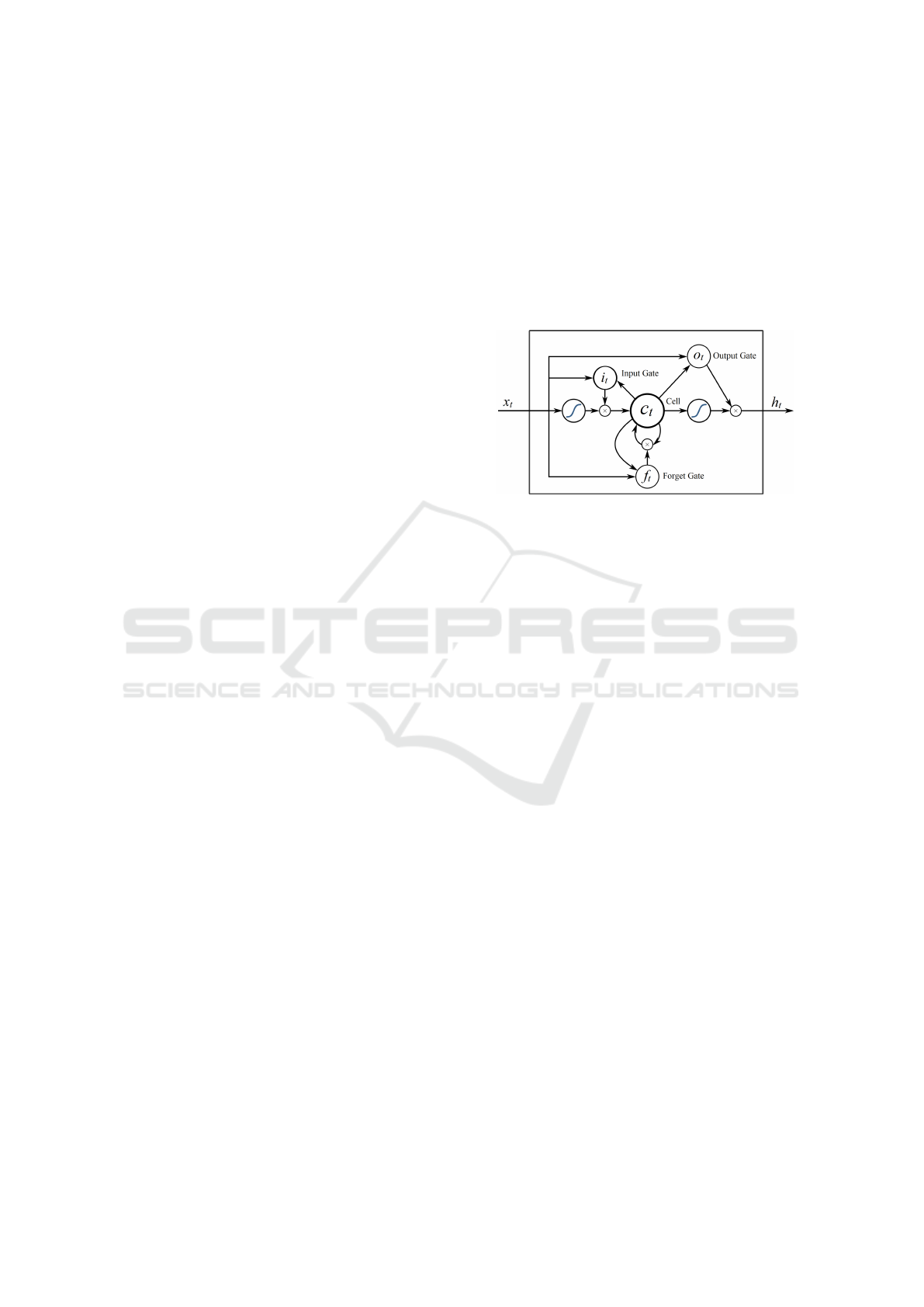
To solve such problems of the recurrent neu-

ral network architecture, Long short-term memory

(LSTM) network was proposed with the idea that

not all inputs in the sequence contribute with impor-

tant information. The LSTM architecture allows the

model to choose which inputs in the sequence are im-

portant and forget the others. A standard LSTM con-

tains an input gate, an output gate and a forget gate as

shown in Figure 1.

Figure 1: LSTM architecture can capture longer input se-

quence.

Let i, f and o denote the input, forget and out-

put gates, respectively. Then, the hidden state h

in a

LSTM network is calculated as follows:

= σ(x

+ h

t−1

+ b

) (1)

= σ(x

+ h

t−1

+ b

) (2)

= σ(x

+ h

t−1

+ b

) (3)

= tanh(x

+ h

t−1

+ b

) (4)

= σ( f

∗C

t−1

+ i

∗

) (5)

= tanh(C

) ∗ o

(6)

In the equations, U is the weight matrix from the input

and W is the weight matrix from the hidden layer in

the previous time step. C

is the memory of the unit

and

is the candidate for cell state at timestamp t. σ

denotes the sigmoid function and ∗ is the elementwise

multiplication.

LSTM models are effective in sequential tasks. In

sequence tagging, (Huang et al., 2015) proposed a

model that processes the feature in both directions.

In speech recognition, (Graves et al., 2013) used the

bidirectional LSTM and achieved state-of-the-art re-

sults in phoneme recognition. In language modeling,

(Sundermeyer et al., 2012) proved that using LSTM

can bring signiﬁcant improvement in this task.

3 PROPOSED APPROACH

Multi-class classiﬁcation is the task of classifying in-

stances into one of K classes and can be trained for

ICAART 2020 - 12th International Conference on Agents and Artiﬁcial Intelligence

sequence prediction (cf. Section 2). For that, a neu-

ral network classiﬁer is given a vectorized represen-

tation of an input and produces a K-dimensional pre-

dicted vector

= [ ˆy

,..., ˆy

], which is a probability

distribution representing the conﬁdence of the clas-

siﬁer over K classes. In the standard training pro-

cess, the network is trained to generate a high conﬁ-

dence towards the correct class by updating its weight

θ to minimize Kullback-Leibler divergence between

its prediction vector

y and the one-hot representation

y of the correct class (cf. Equation 7).

(y,

∑

i=1

log

ˆy

(7)

In general, a target distribution y

= [y

,. ..,y

]

can be deﬁned in term of one-hot representation, i.e.,

the true distribution. However, using the true distribu-

tion as a target distribution can cause a neural network

to gain feedback merely through the predicted conﬁ-

dence of the correct class. The feedback through other

classes, which may be helpful for training, is entirely

disregarded. As exempliﬁed in Section 1, the pre-

dicted conﬁdence for each class indeed provides feed-

back for training unequally. A neural network should

be informed that the mistake of prediction on classes

similar to the target class indeed provides more signif-

icant feedback than the unrelated classes. To incorpo-

rate knowledge about similarity perception between

classes, we propose to involve the following steps at

training time:

1. Initialize a distribution capturing the similarity be-

tween classes (cf. Subsection 3.1),

2. Train progressively from the similarity distribu-

tion to the true distribution (cf. Subsection 3.2).

3.1 Similarity Distribution Initialization

To address how the similarity distribution should be

initialized, we ﬁrst take a look into the literature of

similarity measure. The most basic (but useful) one

was developed by (Tversky, 1977). In Tversky’s

model, an object constitutes a number of properties

(or features). Then, the similarity of two objects is

measured by the relationship between a number of

common properties and a number of different prop-

erties. Nevertheless, not every properties need to be

taken into account for similarity perception. The stud-

ies in (Hesse, 1965; Waller, 2001) reported that prop-

erties involved in similarity perception should be rel-

evant to the context of an application domain. Taking

into account these characteristics, we deﬁne the no-

tion of similarity as follows.

Let P

= {p

, p

,. .., p

} be a set of properties

constituting all classes in the dataset. We denote the

property set of class a by P

, in which P

⊆ P . To

capture the notion of relevancy, we deﬁne a function

w : P → R

≥0

capturing the importance of properties,

in which w(p

) > 0 indicates that p

has more impor-

tance and w(p

)

= 0 indicates that p

is of no impor-

tance in an application context. Then, the similarity

between class a and b (denoted by s(a,b)) can be de-

ﬁned in the following equation.

s(a,b)

∑

p∈P

∩P

w(p) (8)

Intuitively, Equation 8 calculates the summation of

weighted common properties between two classes.

Let s

= [s

,. ..,s

] be a vector representing the

similarity of class a against other classes. Equation

9 expresses an approach to construct arbitrary vector

. Observe that we employ the summation in the de-

nominator part as a normalizing factor.

s(i,k)

∑

j=1

s(i, j)

(9)

To turn a similarity vector into a probability mass

distribution t

= [t

,. ..,t

], we employ the softmax

function as deﬁned in Equation 10. Intuitively, a sim-

ilarity distribution t

captures the similarity of class a

against other classes.

= softmax(s

)

exp(s

/T )

∑

j=1

exp(s

a j

/T )

(10)

where T is a temperature used to control the probabil-

ity mass assigned to a property. Observe that when T

approaches the inﬁnity, the distribution becomes uni-

form. Hence, the common properties shared mostly

among classes contribute a large probability mass. On

the other hand, as T approaches 0, the distribution is

similar to the argmax operation, i.e., it is similar to

one-hot representation. Hence, the unique properties

of constituting classes contribute a large probability

mass.

3.2 Progressive Training with Decay

This subsection proposes a training strategy called

progressive training that enables to train the model

with a similarity distribution and a true distribution.

To handle this style of training properly, we force the

training process to gradually change the target distri-

bution from the similarity distribution to the true dis-

tribution. For that, T must be high at the beginning of

training and periodically be decreased during training.

This training scheme enables the neural network to

learn from common properties at the early stages; and

also, learn from unique properties at the later stages.

Progressive Training in Recurrent Neural Networks for Chord Progression Modeling

Speciﬁcally, we use a scheduler to decrease tem-

perature T

at training epoch t in a similar manner

used by modern stochastic gradient approaches for

decreasing the learning rate. Equation 11 expresses

the scheduler employed in this work.

t−1

1 + λt

(11)

where T

indicates the initial temperature and λ rep-

resents a decay rate. At training epoch t, we generate

a distribution t

of the relevant class a with tempera-

ture T

and update the parameter θ which minimizes

the loss function D

y). We summarize the train-

ing process in Algorithm 1. Furthermore, Figure 2

illustrates a transition of the similarity target distribu-

tion according to each temperature. We also note that

other schedulers also exist (e.g. linear and exponential

decays) which are not engaged in our experiments;

thus, are remained to investigate as future tasks.

Algorithm 1: Progressive learning with class

similarity distribution.

Input : Property set P , weight function w,

initial temperature T

, decay rate λ

Output: Optimal parameter θ

1 Compute similarity vector t

for any class a

using Equation 9

2 Initialize the parameters θ

3 t ← 0

4 while θ

not converged do

5 t ← t + 1

6 Compute temperature T

using Equation 11

7 Compute similarity target t

for class a at

temperature T

using Equation 10

8 Update the parameter θ

to minimize the

loss function D

9 end

4 EXPERIMENTS

In this section, we specify chord properties used

to generate a similarity distribution and demonstrate

the effectiveness of the proposed method on model-

ing chord progression in Beethoven string quartets.

Source code for all experiments is available online

4.1 Dataset

The Annotated Beethoven Corpus (ABC) (Neuwirth

et al., 2018) used in this paper contains harmonic

https://github.com/kienvu58/chord-progression-

modeling

analyses of all sixteen Beethoven string quartets. Six-

teen string quartets (70 movements) were composed

between 1800–1826, comprising Beethoven’s middle

and late creative phrases; and hence, both the high

Classical and early Romantic eras. We split each

piece into phrases and removed continuous chord rep-

etitions in each phrase since we would not model

the duration of each chord. In total, there were 968

phrases with an average length of 21.

We used 5-fold cross-validation and reported the

performance of models in terms of perplexity and ac-

curacy. For each fold, there were about 200 phrases

to evaluate models and remaining phrases were split

into training and validation set. For the training set,

we augmented the data by transposing each phrase

into 12 keys, resulting in the training dataset of about

8000 samples.

For chord vocabulary, we used 273 chord tokens.

Each chord token has two parts: the key and the chord

type. There are 21 keys which are A, B, C, D, E, F, G,

A[, B[, C[, D[, E[, F[, G[, A], B], C], D], E], F], and

G]. Furthermore, there are 13 chord types which are:

major triad, minor triad, augmented triad, diminished

triad, dominant seventh chord, minor seventh chord,

major seventh chord, diminished seventh chord, half-

diminished seventh chord, augmented seventh chord,

Italian augmented sixth chord, German augmented

sixth chord, and French augmented sixth chord.

4.2 Experimental Settings

4.2.1 Chord Properties

In our experiments, we deﬁned according to the music

structure that a chord consists of 6 properties and they

were used to compute the similarity between chords.

These properties are formally given as follows:

P = {token name,key name,key number,

triad form, ﬁgured bass, note pair }

Property token name is the name of the token us-

ing to represent a chord. If property token name is

the only property in the set P , then this is equivalent

to using a one-hot representation as a target distribu-

tion.

Property key name is the name of a chord key,

which takes one of 21 values mentioning in the previ-

ous section.

Property key number is the value of the chord key,

which is a number from 0 to 11. If two chords have

the same key number but the different key name, then

their keys are enharmonic. For example, F] and G[

are enharmonic keys.

Property triad form is the chord form of the ﬁrst

three notes in a chord. There are four kinds of

ICAART 2020 - 12th International Conference on Agents and Artiﬁcial Intelligence

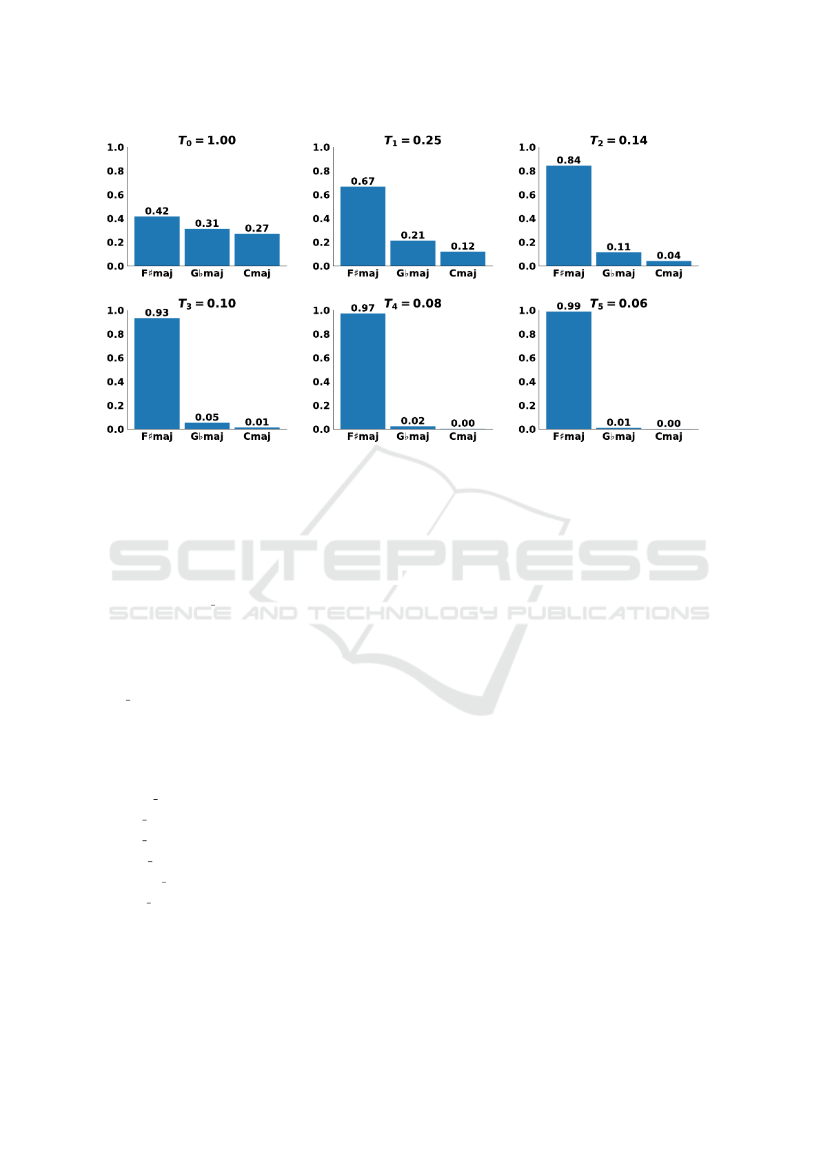
Figure 2: Transition of a similarity target distribution according to each temperature. The initial temperature is T

= 1.00 and

the decay rate is λ

= 3.00. The similarity target gradually becomes a one-hot representation.

chord form, namely minor, major, diminished, or aug-

mented form. Each chord form produces a different

musical effect. For instance, the major form is gen-

erally perceived as positive-sounding and the minor

is generally perceived as negative-sounding (Bakker

and Martin, 2015; Gagnon and Peretz, 2003).

Property ﬁgured bass is used to categorize a chord

into a triad, a seventh, or an augmented sixth. Each of

these chord types has a different role in a chord pro-

gression. For example, augmented sixth chords are

usually used as a predominant function.

Furthermore, each chord can have multiple

note pair properties, which are note pairs created

from the chord note set.

Finally, we exemplify the identiﬁcation of a chord

according to these properties, For example, C domi-

nant seventh chord contains 4 notes C(0), E(4), G(7),

B[(10). It has the following properties:

• token name: C7

• key number: 0

• key name: C

• triad

form: major

• ﬁgured bass: 7

• note pair: (0, 4), (0, 7), (0, 10) (4, 7), (4, 10), (7,

10)

4.2.2 Temperature Decay Conﬁgurations

As proposed in Section 3.2, we periodically update

similarity distributions during the training stage us-

ing Equation 11. To ﬁnd optimal values of the initial

temperature and decay rate, we grid-search the initial

temperature in {0.01,0.025,0.05,0.0075,0.1} and

the decay rate in {0.0005,0.001, 0.0025,0.005, 0.01}.

Also, we compared the performance of models

when training with similarity distributions generated

from ﬁxed temperatures and scheduled temperatures.

We sampled 10 ﬁxed temperatures from the schedul-

ing equation (Equation 11).

4.2.3 Model Conﬁgurations

We investigated the effectiveness of the proposed

method on an LSTM-based neural network, consist-

ing of 3 layers: embedding, recurrent, and fully-

connected layers. We used Adam optimizer (Kingma

and Ba, 2014) with the learning rate of 0.001 and de-

fault hyper-parameters suggested by the authors. For

all experiments, the maximum number of epochs was

set to 200, and early stopping with the patience value

of 10 was used to prevent over-ﬁtting. All hyper-

parameter settings are summarized in Table 1.

4.3 Experimental Results

4.3.1 One-hot vs. Similarity Distributions

Table 2 shows the performance of models training

with similarity distributions and one-hot distributions.

In this experiment, we used the same weight for all

chord properties and different initial temperatures and

decay rates to generate similarity distributions.

Progressive Training in Recurrent Neural Networks for Chord Progression Modeling

Table 1: Hyper-parameter settings for all experiments.

Hyper-parameter Setting

Embedding

Embedding size 128

Recurrent cells

LSTM hidden size 128

Fully-connected

Number of layers 1

Fully-connected hidden size 128

Training

Optimizer Adam

Learning rate α 0.001

0.9

0.999

ε 10

−8

Batch size 32

Maximum number of epochs 200

Early stopping patience 10

In general, the performance of all models training

with similarity distributions is better than one train-

ing with one-hot distributions. The highest accuracy

is 0.71, which is about 29% higher than the model

training with one-hot distributions. The lowest per-

plexity is 2.44, which is about 30% lower.

Moreover, there is a relation between the magni-

tude of initial temperatures and decay rates in the re-

sults. When the initial temperature is high, using large

decay rates produce a better model and vice versa.

This suggests that we can ﬁx a reasonable initial tem-

perature and grid-search for an optimal decay rate.

This reduces the search space of hyper-parameters.

4.3.2 Fixed vs. Scheduled Temperature

Table 3 and Table 4 show the performance of mod-

els training with ﬁxed and scheduled temperatures in

terms of accuracy and perplexity. The ﬁrst column

in these tables shows the property weight set used

to generate similarity distribution and the headers’ ti-

tle indicates the temperature values. We used Equa-

tion 11 with T

= 0.05 and λ = 0.001 to schedule the

temperature. We sampled temperatures at 10 time-

steps with the interval value of 20 to generate ﬁxed

similarity distributions.

In general, models training with scheduled tem-

peratures have better performance than ones train-

ing with ﬁxed temperatures. At ﬁxed temperature

settings, models training with high temperatures had

worse performance than ones training with low tem-

peratures. The reason is similarity distributions gen-

erated with high temperatures have higher entropy,

thus models ﬁtting these distributions tend to produce

Table 2: Performance of models training with uniform

weight set (1, 1, 1, 1, 1, 1).

λ accuracy perplexity

0.1 0.01 0.68 2.60

0.1 0.005 0.71 2.47

0.1 0.0025 0.71 2.50

0.1 0.001 0.69 2.57

0.1 0.0005 0.66 2.77

0.075 0.01 0.70 2.44

0.075 0.005 0.69 2.55

0.075 0.0025 0.71 2.48

0.075 0.001 0.68 2.62

0.075 0.0005 0.67 2.71

0.05 0.01 0.67 2.55

0.05 0.005 0.70 2.46

0.05 0.0025 0.70 2.50

0.05 0.001 0.71 2.49

0.05 0.0005 0.64 2.93

0.025 0.01 0.63 2.73

0.025 0.005 0.64 2.73

0.025 0.0025 0.70 2.46

0.025 0.001 0.70 2.53

0.025 0.0005 0.69 2.59

0.01 0.01 0.56 3.19

0.01 0.005 0.55 3.31

0.01 0.0025 0.58 3.04

0.01 0.001 0.64 2.67

0.01 0.0005 0.66 2.64

Train with one-hot 0.55 3.48

more random predictions.

Also, we investigated the effect of individual

properties in contribution to the performance of mod-

els. We specify the weight of each property in a

6-dimension tuple, each dimension is correspond-

ing to one of six properties: token

name, key name,

triad form, ﬁgured bass, and note pair respectively.

We used only two properties once at a time, with

one of them is property token name since this is the

unique property to distinguish chords from each other.

We ﬁxed the weight of the property token name with

a value of 16 and grid-searched the weight of the other

property in {2, 4,8, 16,32}. Weights of unused prop-

erties were set to zeros.

The results show that the models training with

similarity distributions generated using two properties

token name and note pair have better performance

than others on average. This could be expected since

intuitively the property note pair encodes more infor-

mation than other properties. Also, similarity distri-

butions generated from all properties probably still

ICAART 2020 - 12th International Conference on Agents and Artiﬁcial Intelligence

Table 3: Accuracy of models training with ﬁxed and scheduled temperature.

Properties’ Weight Scheduled 5.00E-02 4.06E-02 2.23E-02 8.31E-03 2.13E-03 3.77E-04 4.63E-05 3.98E-06 2.41E-07 1.04E-08

(16, 0, 0, 0, 0, 1) 0.57 0.38 0.41 0.52 0.55 0.55 0.54 0.54 0.54 0.55 0.53

(16, 0, 0, 0, 0, 2) 0.68 0.33 0.34 0.45 0.54 0.54 0.55 0.54 0.54 0.54 0.54

(16, 0, 0, 0, 0, 4) 0.69 0.26 0.31 0.37 0.54 0.55 0.54 0.53 0.55 0.55 0.54

(16, 0, 0, 0, 0, 8) 0.70 0.26 0.26 0.37 0.51 0.54 0.54 0.54 0.55 0.54 0.55

(16, 0, 0, 0, 0, 16) 0.70 0.19 0.26 0.35 0.47 0.54 0.54 0.55 0.52 0.54 0.55

(16, 0, 0, 0, 0, 32) 0.70 0.16 0.20 0.31 0.43 0.54 0.55 0.55 0.54 0.54 0.55

(16, 0, 0, 0, 1, 0) 0.61 0.39 0.39 0.52 0.55 0.53 0.54 0.55 0.54 0.54 0.54

(16, 0, 0, 0, 2, 0) 0.68 0.26 0.30 0.40 0.54 0.54 0.55 0.55 0.54 0.54 0.54

(16, 0, 0, 0, 4, 0) 0.69 0.10 0.11 0.31 0.47 0.53 0.54 0.55 0.55 0.53 0.54

(16, 0, 0, 0, 8, 0) 0.67 0.08 0.08 0.14 0.43 0.54 0.54 0.54 0.54 0.54 0.54

(16, 0, 0, 0, 16, 0) 0.64 0.07 0.07 0.09 0.22 0.48 0.54 0.55 0.55 0.54 0.54

(16, 0, 0, 0, 32, 0) 0.65 0.06 0.07 0.08 0.12 0.46 0.55 0.55 0.53 0.54 0.53

(16, 0, 0, 1, 0, 0) 0.56 0.43 0.49 0.55 0.54 0.54 0.55 0.55 0.54 0.55 0.54

(16, 0, 0, 2, 0, 0) 0.67 0.37 0.45 0.49 0.54 0.54 0.55 0.54 0.54 0.54 0.54

(16, 0, 0, 4, 0, 0) 0.68 0.18 0.26 0.42 0.53 0.53 0.55 0.54 0.54 0.55 0.54

(16, 0, 0, 8, 0, 0) 0.67 0.15 0.10 0.24 0.49 0.55 0.54 0.54 0.53 0.55 0.54

(16, 0, 0, 16, 0, 0) 0.66 0.08 0.09 0.13 0.40 0.53 0.54 0.54 0.53 0.55 0.55

(16, 0, 0, 32, 0, 0) 0.65 0.07 0.08 0.10 0.18 0.46 0.55 0.54 0.54 0.54 0.55

(16, 0, 1, 0, 0, 0) 0.54 0.55 0.55 0.54 0.55 0.54 0.55 0.54 0.54 0.54 0.54

(16, 0, 2, 0, 0, 0) 0.53 0.50 0.53 0.53 0.54 0.53 0.54 0.55 0.54 0.55 0.53

(16, 0, 4, 0, 0, 0) 0.55 0.37 0.43 0.54 0.54 0.55 0.55 0.54 0.55 0.54 0.54

(16, 0, 8, 0, 0, 0) 0.59 0.31 0.32 0.46 0.54 0.54 0.53 0.55 0.55 0.54 0.54

(16, 0, 16, 0, 0, 0) 0.65 0.25 0.27 0.38 0.51 0.54 0.54 0.54 0.54 0.55 0.54

(16, 0, 32, 0, 0, 0) 0.65 0.24 0.26 0.34 0.48 0.55 0.53 0.55 0.54 0.55 0.55

(16, 1, 0, 0, 0, 0) 0.53 0.55 0.54 0.55 0.55 0.54 0.55 0.54 0.53 0.54 0.54

(16, 2, 0, 0, 0, 0) 0.54 0.55 0.54 0.54 0.55 0.54 0.55 0.54 0.55 0.55 0.53

(16, 4, 0, 0, 0, 0) 0.54 0.52 0.54 0.54 0.55 0.54 0.54 0.54 0.54 0.54 0.54

(16, 8, 0, 0, 0, 0) 0.56 0.40 0.44 0.54 0.54 0.55 0.51 0.54 0.54 0.54 0.54

(16, 16, 0, 0, 0, 0) 0.59 0.36 0.40 0.51 0.54 0.54 0.54 0.54 0.55 0.55 0.55

(16, 32, 0, 0, 0, 0) 0.60 0.31 0.35 0.45 0.53 0.55 0.54 0.54 0.55 0.54 0.53

(1, 1, 1, 1, 1, 1) 0.71 0.10 0.10 0.26 0.40 0.54 0.55 0.54 0.55 0.54 0.55

Table 4: Perplexity of models training with ﬁxed and scheduled temperature.

Properties’ Weight Scheduled 5.00E-02 4.06E-02 2.23E-02 8.31E-03 2.13E-03 3.77E-04 4.63E-05 3.98E-06 2.41E-07 1.04E-08

(16, 0, 0, 0, 0, 1) 3.19 32.86 19.17 5.06 3.47 3.49 3.51 3.56 3.53 3.51 3.74

(16, 0, 0, 0, 0, 2) 2.54 73.81 55.23 12.79 3.65 3.52 3.50 3.61 3.78 3.63 3.56

(16, 0, 0, 0, 0, 4) 2.50 109.18 89.79 37.77 4.27 3.51 3.56 3.80 3.47 3.51 3.65

(16, 0, 0, 0, 0, 8) 2.46 121.70 114.00 61.17 7.40 3.58 3.65 3.62 3.52 3.53 3.48

(16, 0, 0, 0, 0, 16) 2.45 133.34 117.52 76.82 14.45 3.81 3.60 3.50 3.98 3.66 3.46

(16, 0, 0, 0, 0, 32) 2.44 135.78 124.38 84.53 20.14 5.13 3.51 3.52 3.57 3.55 3.46

(16, 0, 0, 0, 1, 0) 2.87 42.33 28.85 5.43 3.48 3.70 3.59 3.49 3.65 3.52 3.57

(16, 0, 0, 0, 2, 0) 2.59 100.39 80.88 26.54 3.79 3.60 3.46 3.46 3.65 3.59 3.56

(16, 0, 0, 0, 4, 0) 2.59 138.53 132.11 75.39 9.41 3.73 3.53 3.53 3.48 3.73 3.61

(16, 0, 0, 0, 8, 0) 2.71 144.80 142.20 119.56 33.43 3.65 3.62 3.60 3.53 3.54 3.62

(16, 0, 0, 0, 16, 0) 3.03 147.71 143.68 129.42 78.43 7.56 3.55 3.52 3.47 3.55 3.70

(16, 0, 0, 0, 32, 0) 2.91 147.03 143.16 131.12 94.99 24.03 3.46 3.46 3.87 3.61 3.74

(16, 0, 0, 1, 0, 0) 3.34 15.90 8.25 3.50 3.61 3.57 3.40 3.48 3.54 3.46 3.60

(16, 0, 0, 2, 0, 0) 2.55 52.35 23.36 7.21 3.65 3.57 3.54 3.61 3.55 3.65 3.58

(16, 0, 0, 4, 0, 0) 2.67 113.22 89.94 29.01 3.90 3.66 3.53 3.57 3.62 3.44 3.55

(16, 0, 0, 8, 0, 0) 2.73 117.66 127.01 78.11 9.31 3.48 3.62 3.55 3.90 3.43 3.60

(16, 0, 0, 16, 0, 0) 2.85 137.28 129.85 102.09 28.62 3.77 3.64 3.60 3.82 3.50 3.49

(16, 0, 0, 32, 0, 0) 2.91 138.28 132.57 106.69 56.22 8.10 3.49 3.59 3.63 3.56 3.48

(16, 0, 1, 0, 0, 0) 3.68 3.82 3.59 3.54 3.43 3.61 3.52 3.57 3.50 3.56 3.52

(16, 0, 2, 0, 0, 0) 3.93 7.98 4.98 3.75 3.60 3.98 3.53 3.46 3.66 3.48 3.74

(16, 0, 4, 0, 0, 0) 3.46 28.21 16.40 4.10 3.55 3.48 3.49 3.54 3.52 3.65 3.53

(16, 0, 8, 0, 0, 0) 3.00 63.37 46.70 11.80 3.68 3.61 3.87 3.48 3.53 3.52 3.61

(16, 0, 16, 0, 0, 0) 2.66 97.26 80.50 28.65 5.02 3.55 3.55 3.60 3.57 3.49 3.64

(16, 0, 32, 0, 0, 0) 2.64 108.11 93.90 48.26 9.78 3.54 3.69 3.52 3.59 3.42 3.44

(16, 1, 0, 0, 0, 0) 3.66 3.44 3.64 3.48 3.50 3.65 3.47 3.67 4.10 3.61 3.53

(16, 2, 0, 0, 0, 0) 3.51 3.71 3.62 3.57 3.47 3.56 3.43 3.58 3.47 3.52 3.80

(16, 4, 0, 0, 0, 0) 3.55 6.83 4.38 3.55 3.44 3.59 3.70 3.55 3.63 3.65 3.61

(16, 8, 0, 0, 0, 0) 3.27 26.90 14.02 3.82 3.56 3.49 4.25 3.53 3.63 3.54 3.60

(16, 16, 0, 0, 0, 0) 3.01 53.50 35.36 7.15 3.58 3.64 3.61 3.56 3.50 3.50 3.48

(16, 32, 0, 0, 0, 0) 2.96 72.86 54.11 16.19 4.17 3.53 3.56 3.56 3.54 3.62 3.78

(1, 1, 1, 1, 1, 1) 2.49 159.26 145.45 112.62 38.33 3.88 3.51 3.56 3.51 3.63 3.43

Progressive Training in Recurrent Neural Networks for Chord Progression Modeling

produce better models than similarity distributions

generated from two individual properties.

To further investigate, we chose the best weight

(in terms of accuracy then perplexity) for each prop-

erty in these experiments and combined them into the

weight set (16,32,16,4,4,32). Table 5 shows the per-

formance of models training with this weight set. The

best perplexity and accuracy are 2.39 and 0.71 respec-

tively. This is slightly better than training with a uni-

form weight set. This means we probably do not need

to search for an optimal weight set but can still get a

signiﬁcant improvement when comparing to training

with one-hot distributions.

Table 5: Performance of models training with weight set

(16, 32, 16, 4, 4, 32).

λ accuracy perplexity

0.1 0.01 0.58 3.21

0.1 0.005 0.59 3.13

0.1 0.0025 0.58 3.32

0.1 0.001 0.59 3.17

0.1 0.0005 0.57 3.23

0.075 0.01 0.71 2.41

0.075 0.005 0.71 2.42

0.075 0.0025 0.63 2.79

0.075 0.001 0.60 2.99

0.075 0.0005 0.59 3.11

0.05 0.01 0.66 2.70

0.05 0.005 0.70 2.45

0.05 0.0025 0.69 2.52

0.05 0.001 0.69 2.47

0.05 0.0005 0.61 2.91

0.025 0.01 0.64 2.87

0.025 0.005 0.66 2.65

0.025 0.0025 0.68 2.55

0.025 0.001 0.71 2.39

0.025 0.0005 0.66 2.58

0.01 0.01 0.62 2.95

0.01 0.005 0.66 2.68

0.01 0.0025 0.64 3.31

0.01 0.001 0.68 2.59

0.01 0.0005 0.63 2.81

5 RELATED WORK

Most of the literature on enhancing learning’s efﬁ-

ciency relies on the idea of exploiting much knowl-

edge at training; for instance, transfer learning, multi-

task learning, knowledge compilation, and curriculum

learning. We review each of them as follows.

In transfer learning, two different application do-

mains (called the source and the target) are consid-

ered, in which its main purpose is to utilize the learnt

parameters from the source domain into the target

problem. Efforts on this issue have been made in sev-

eral areas such as computer vision (cf. (Krizhevsky

et al., 2012) for an example of pre-trained model

on ImageNet) and natural language processing (cf.

Word2Vec (Mikolov et al., 2013; Pennington et al.,

2014) for the word embedding using neural net-

works). Approaches similar to Word2Vec can be also

applied to learn vector-based representations from

structured knowledge like ontologies and knowledge

graph. For instance, (Ristoski et al., 2019) exploited

medical ontologies to improve the quality of the learnt

representations and prediction performance. Despite

their promising results, this approach requires a large

volume of the source dataset.

Multi-task learning aims at leveraging the inter-

class relationship at training time. For instance, (Vu-

ral et al., 2009) developed a multi-class large margin

classiﬁer that extracts and takes advantage of class re-

lationships. For the subject of video classiﬁcation,

(Wu et al., 2014) learned feature relationships and ex-

ploited the class relationship in a neural network to

improve the prediction.

Knowledge can be compiled and distilled to a tar-

get problem. For instance, (Hinton et al., 2015) as-

sumed that two different models (called a teacher

model and a student model) do exist and proposed a

technique for distilling the knowledge of the teacher

model to the student model. Indeed, the authors

aimed at developing a compression technique in a

sense that the teacher model is an ensemble of many

models or a large highly regularized model and the

student model can be a smaller one. This technique

can be also used as a regularization method such that a

target model can imitate a source model to avoid over-

ﬁtting (cf. (Asami et al., 2017)). Furthermore, when

categorical information is available for compilation,

feature vectors can also be built from similarity across

categories. For instance, (Cerda et al., 2018) proposed

a similarity encoding approach to obtain a better rep-

resentation of categorical variables, especially in the

presence of dirty categorical data.

In curriculum learning, two different kinds of

training examples, viz. the easy ones and the difﬁ-

cult ones, are considered at training time. Then, this

approach starts the training from easy examples and

gradually increase the difﬁculty of learning by train-

ing with difﬁcult examples. For instance, (Bengio

et al., 2015) employed this style of learning for se-

quence prediction, in which the easy examples were

the known tokens and the difﬁcult examples were the

ICAART 2020 - 12th International Conference on Agents and Artiﬁcial Intelligence

realistic ones provided by the model itself. The au-

thors also showed that several sequence prediction

tasks could yield performance improvements and did

not incur longer training times.

Considering the interclass relationship and sched-

uled learning, our approach is similar to multi-task

learning and curriculum learning. However, our

method differs from those in the sense that the domain

knowledge about classes’ structure is used to con-

struct the similarity target distribution and the train-

ing objective is forced to go from the similarity dis-

tribution to the true distribution. Indeed, the domain

knowledge about similarity is used to penalize the

model when a wrong-but-not-totally-incorrect predic-

tion has been made. Experiments in chord progress

modeling were conduced to warrant our investigation.

6 CONCLUSION

This paper introduces an approach to incorporate the

domain knowledge about class similarity at training

time. For that, we deﬁne similarity as weighted com-

mon properties and propose a learning strategy called

progressive training for enabling the model to learn

from both a similarity distribution and the true distri-

bution during training. Speciﬁcally, instead of consid-

ering merely one-hot encoding, our method leverages

interclass similarity encoding by utilizing the temper-

ature during the training phase. Our experiments on

chord progression reveal that our proposed approach

can yield predictive performance improvement with-

out incurring longer training time.

It is worth observing that the idea proposed in this

work is general enough in such a way that it should

be applicable to a variety of common tasks; for in-

stance, classes in CIFAR-10

are somewhat hierar-

chical; also, certain words in the embedding space

are distinguishable whether they are similar or not.

Hence, it is a natural step for us to extend the exper-

iments to these tasks. Another interesting direction

involves further investigation on the automatic con-

struction of similarity encoding, as well as exploring

alternative methods for scheduling strategies and sim-

ilarity distance functions.

REFERENCES

Asami, T., Masumura, R., Yamaguchi, Y., Masataki, H., and

Aono, Y. (2017). Domain adaptation of dnn acoustic

https://www.cs.toronto.edu/∼kriz/cifar.html

models using knowledge distillation. In 2017 IEEE In-

ternational Conference on Acoustics, Speech and Sig-

nal Processing (ICASSP), pages 5185–5189.

Bahdanau, D., Cho, K., and Bengio, Y. (2015). Neural

machine translation by jointly learning to align and

translate. In 3rd International Conference on Learn-

ing Representations, ICLR 2015, San Diego, CA, USA,

May 7-9, 2015, Conference Track Proceedings.

Bakker, D. R. and Martin, F. H. (2015). Musical chords

and emotion: Major and minor triads are processed

for emotion. Cognitive, Affective, & Behavioral Neu-

roscience, 15(1):15–31.

Bengio, S., Vinyals, O., Jaitly, N., and Shazeer, N. (2015).

Scheduled sampling for sequence prediction with re-

current neural networks. In Proceedings of the 28th

International Conference on Neural Information Pro-

cessing Systems - Volume 1, NIPS’15, pages 1171–

1179, Cambridge, MA, USA. MIT Press.

Cerda, P., Varoquaux, G., and K

egl, B. (2018). Similarity

encoding for learning with dirty categorical variables.

Machine Learning, 107(8):1477–1494.

Cho, K., Van Merri

enboer, B., Gulcehre, C., Bahdanau, D.,

Bougares, F., Schwenk, H., and Bengio, Y. (2014).

Learning phrase representations using rnn encoder-

decoder for statistical machine translation. arXiv

preprint arXiv:1406.1078.

Choi, K., Fazekas, G., and Sandler, M. B. (2016). Text-

based LSTM networks for automatic music composi-

tion. CoRR, abs/1604.05358.

Gagnon, L. and Peretz, I. (2003). Mode and tempo relative

contributions to “happy-sad” judgements in equitone

melodies. Cognition and emotion, 17(1):25–40.

Graves, A., Mohamed, A.-r., and Hinton, G. (2013).

Speech recognition with deep recurrent neural net-

works. In 2013 IEEE international conference on

acoustics, speech and signal processing, pages 6645–

6649. IEEE.

Hesse, M. B. (1965). Models and analogies in science.

Hinton, G., Vinyals, O., and Dean, J. (2015). Distilling

the knowledge in a neural network. arXiv preprint

arXiv:1503.02531.

Hochreiter, S. and Schmidhuber, J. (1997). Long short-term

memory. Neural computation, 9(8):1735–1780.

Huang, Z., Xu, W., and Yu, K. (2015). Bidirectional

lstm-crf models for sequence tagging. arXiv preprint

arXiv:1508.01991.

John, J. H. (1982). Neural network and physical systems

with emergent collective computational abilities. Pro-

ceedings of the National Academy of Sciences of the

United States of America, 79:2554–2558.

Kingma, D. P. and Ba, J. (2014). Adam: A

method for stochastic optimization. arXiv preprint

arXiv:1412.6980.

Krizhevsky, A., Sutskever, I., and Hinton, G. E. (2012). Im-

agenet classiﬁcation with deep convolutional neural

networks. In Advances in Neural Information Pro-

cessing Systems 25: 26th Annual Conference on Neu-

ral Information Processing Systems 2012. Proceed-

ings of a meeting held December 3-6, 2012, Lake

Tahoe, Nevada, United States., pages 1106–1114.

Progressive Training in Recurrent Neural Networks for Chord Progression Modeling

Meng, F. and Zhang, J. (2019). DTMT: A novel deep tran-

sition architecture for neural machine translation. In

The Thirty-Third AAAI Conference on Artiﬁcial Intel-

ligence, AAAI 2019, The Thirty-First Innovative Ap-

plications of Artiﬁcial Intelligence Conference, IAAI

2019, The Ninth AAAI Symposium on Educational

Advances in Artiﬁcial Intelligence, EAAI 2019, Hon-

olulu, Hawaii, USA, January 27 - February 1, 2019.,

pages 224–231.

Mikolov, T., Chen, K., Corrado, G., and Dean, J. (2013).

Efﬁcient estimation of word representations in vector

space. arXiv preprint arXiv:1301.3781.

Neuwirth, M., Harasim, D., Moss, F. C., and Rohrmeier,

M. (2018). The Annotated Beethoven Corpus (ABC):

A Dataset of Harmonic Analyses of All Beethoven

String Quartets. Frontiers in Digital Humanities, 5:16.

Pennington, J., Socher, R., and Manning, C. (2014). Glove:

Global vectors for word representation. In Proceed-

ings of the 2014 Conference on Empirical Methods in

Natural Language Processing (EMNLP), pages 1532–

1543, Doha, Qatar. Association for Computational

Linguistics.

Ristoski, P., Rosati, J., Noia, T. D., Leone, R. D., and Paul-

heim, H. (2019). Rdf2vec: RDF graph embeddings

and their applications. Semantic Web, 10(4):721–752.

Song, L., Cheong, C. W., Yin, K., Cheung, W. K., Fung,

B. C. M., and Poon, J. (2019). Medical concept em-

bedding with multiple ontological representations. In

Proceedings of the Twenty-Eighth International Joint

Conference on Artiﬁcial Intelligence, IJCAI-19, pages

4613–4619. International Joint Conferences on Artiﬁ-

cial Intelligence Organization.

Sundermeyer, M., Schl

uter, R., and Ney, H. (2012). Lstm

neural networks for language modeling. In Thirteenth

annual conference of the international speech commu-

nication association.

Sutskever, I., Vinyals, O., and Le, Q. V. (2014). Sequence to

sequence learning with neural networks. In Proceed-

ings of the 27th International Conference on Neural

Information Processing Systems - Volume 2, NIPS’14,

pages 3104–3112, Cambridge, MA, USA. MIT Press.

Tversky, A. (1977). Features of similarity. Psychological

review, 84(4):327.

Vinyals, O., Toshev, A., Bengio, S., and Erhan, D. (2015).

Show and tell: A neural image caption generator. In

IEEE Conference on Computer Vision and Pattern

Recognition, CVPR 2015, Boston, MA, USA, June 7-

12, 2015, pages 3156–3164.

Vural, V., Fung, G., Rosales, R., and Dy, J. G. (2009).

Multi-class classiﬁers and their underlying shared

structure. In IJCAI.

Waller, B. N. (2001). Classifying and analyzing analogies.

Informal Logic, 21(3).

Wu, Z., Jiang, Y.-G., Wang, J., Pu, J., and Xue, X. (2014).

Exploring inter-feature and inter-class relationships

with deep neural networks for video classiﬁcation. In

Proceedings of the 22Nd ACM International Confer-

ence on Multimedia, MM ’14, pages 167–176, New

York, NY, USA. ACM.

ICAART 2020 - 12th International Conference on Agents and Artiﬁcial Intelligence