A Comparison of Visual Navigation Approaches based on Localization

and Reinforcement Learning in Virtual and Real Environments

Marco Rosano

1,2

, Antonino Furnari

, Luigi Gulino

and Giovanni Maria Farinella

Universit

a degli Studi di Catania, Catania, Italy

OrangeDev s.r.l., via Vasco de Gama 91, Firenze, Italy

Keywords:

Visual Navigation, Reinforcement Learning, Image-based Localization, First Person Vision.

Abstract:

Visual navigation algorithms allow a mobile agent to sense the environment and autonomously ﬁnd its way

to reach a target (e.g. an object in the environment). While many recent approaches tackled this task using

reinforcement learning, which neglects any prior knowledge about the environments, more classic approaches

strongly rely on self-localization and path planning. In this study, we compare the performance of single-

target and multi-target visual navigation approaches based on the reinforcement learning paradigm, and simple

baselines which rely on image-based localization. Experiments performed on discrete-state environments

of different sizes, comprised of both real and virtual images, show that the two paradigms tend to achieve

complementary results, hence suggesting that a combination of the two approaches to visual navigation may

be beneﬁcial.

1 INTRODUCTION

In robotics, one of the most required ability for an

intelligent robot that has to operate in a given envi-

ronment is to autonomously navigate inside it with a

certain degree of accuracy. While humans can eas-

ily navigate in a wide variety of spaces and adapt to

unseen environments, the autonomous robot naviga-

tion problem is still unsolved, even if several meth-

ods have been proposed over the years. Classic “map-

based” approaches to visual navigation generally need

1) the construction of an explicit map of the environ-

ment and 2) a path planning strategy to exploit the

acquired knowledge (Thrun et al., 2005).

To avoid the limitations of map-based approaches,

recent works have tackled the navigation problem

considering “map-less” methods , which only con-

sider a form of implicit representation of the geom-

etry of the space, usually obtained using Convolution

Neural Networks (CNNs) directly trained on images

of the environment (Mirowski et al., 2016; Zhu et al.,

2017; Gupta et al., 2017). In particular, Deep Rein-

forcement Learning (DRL) models recently emerged

as promising methods to learn navigation policies in

a end-to-end manner (Mirowski et al., 2016; Zhu

et al., 2017). Such methods consider high dimen-

sional data as input (often in the form of images)

and return the actions required to reach a speciﬁc tar-

get location. While we would expect DRL naviga-

tion approaches to be applied to real world contexts,

due to the learning-by-simulation approach imposed

by reinforcement learning, most research studies fo-

cus on simulated data (Mnih et al., 2013; Mirowski

et al., 2016; Kempka et al., 2016), even able to recre-

ate the appearance of real environments from images

and to emulate interactions with the agent (i.e. colli-

sions) (Xia et al., 2018; Savva et al., 2019). Despite

such efforts, the substantial domain gap between real

and simulated environments can harm the ability of

these approaches to generalize to real environments.

In this paper, we compare map-based and map-

less visual navigation approaches considering both

single-target and multi-target settings. The consid-

ered map-based algorithms rely on a simple image-

retrieval localization approach (Orlando et al., 2019)

coupled with a path planning routine based on the

computation of the shortest path between the cur-

rent and target locations. The considered map-less

approaches are based on reinforcement learning and

consider both single (Konda and Tsitsiklis, 2000;

Mnih et al., 2016) and multi-target variants (Zhu

et al., 2017). We performed the experiments in envi-

ronments comprising both real and simulated images,

characterized by different sizes, varying the number

of target states to be reached. In the case of multi-

target methods, we tested the generalization ability to

navigate to target states at given distances from the

628

Rosano, M., Furnari, A., Gulino, L. and Farinella, G.

A Comparison of Visual Navigation Approaches based on Localization and Reinforcement Learning in Virtual and Real Environments.

DOI: 10.5220/0008950806280635

In Proceedings of the 15th International Joint Conference on Computer Vision, Imaging and Computer Graphics Theory and Applications (VISIGRAPP 2020) - Volume 5: VISAPP, pages

628-635

ISBN: 978-989-758-402-2; ISSN: 2184-4321

ones seen during training. We report results in terms

of success rate (whether the agent can reach the tar-

get in a limited number of steps) and average num-

ber of steps required to reach the target state. The

considered approaches are compared with respect to

two baselines: an ORacle agent (OR), which always

follows the optimal path to the target state, and a Ran-

dom Walker agent (RW), which follows a random pol-

icy to reach the target.

The results highlight that map-less approaches

based on Reinforcement Learning can achieve op-

timal performances when navigating to targets seen

during training, but are limited when it comes to gen-

eralizing to unseen targets and scaling to large envi-

ronments. Map-based approaches based on localiza-

tion obtain encouraging and complementary results,

despite the poor performance of the localization mod-

ule alone, which suggests that combining approaches

based on RL and localization can be beneﬁcial.

The remainder of the paper is organized as fol-

lows. Section 2 describes the related works. In Sec-

tion 3, we describe the compared approaches. Exper-

imental settings are discussed in Section 4 and results

in Section 5. Section 6 concludes the paper and dis-

cusses future works.

2 RELATED WORKS

Previous works have investigated visual navigation

according to two main settings: map-based and map-

less. Map-based navigation relies on a map of the en-

vironment either created beforehand or built on the

ﬂy during navigation. Map-less navigation relies on

Deep Neural Networks to extract an implicit repre-

sentation of the world from images or other sensory

input. This representation is then used to perform

the navigation task. The learning process can be per-

formed using Imitation Learning (IL) and Reinforce-

ment Learning (RL) as discussed in the following.

Map-based Visual Navigation. Methods falling into

this category assume a map of the environment to

be known and employ path planning (Hong Zhang

and Ostrowski, 2002) or obstacle avoidance algo-

rithms (Ulrich and Borenstein, 1998) to navigate to

the destination. Convolutional Networks have been

also used to create a top-down spatial memory from

ﬁrst-person views (Gupta et al., 2017) or to local-

ize the agent using image-based localization tech-

niques (Kendall et al., 2015; Orlando et al., 2019),

and then apply a path-planning algorithm to ﬁnd the

optimal route to the target.

Image-based Localization. Image-based localiza-

tion plays a central role in the task of sensing an envi-

ronment by an autonomous robot. Localization meth-

ods based on classiﬁcation usually discretize the envi-

ronment by dividing it into classes and address local-

ization as a classiﬁcation task (Ragusa et al., 2019).

Despite the good performances of these approaches,

they are not able to provide an accurate estimation

of the camera pose. Image-retrieval methods rely on

image representation techniques (J

egou et al., 2010;

Arandjelovic et al., 2016) and reduce the pose esti-

mation problem to a nearest neighbor search in the

feature space (Orlando et al., 2019). Image local-

ization can also be tackled as a regression problem,

where a CNN is used to directly estimate the cam-

era pose from images (Kendall et al., 2015). 2D-3D

matching approaches start by extracting 2D feature

points from images, then create a correspondence be-

tween these 2D points and 3D points of a given model

of the scene. The 3D model could be known be-

forehand (Sattler et al., 2016) or incrementally con-

structed (Schnberger and Frahm, 2016).

Map-less Visual Navigation based on Imitation

Learning. These approaches allow to plan the se-

quence of actions to be performed directly from raw

images of the environment, taking advantage of the

ability to learn deep models end-to-end. In Imi-

tation Learning, the policy is obtained from expert

demonstrations, as in a classic supervised learning

setup (Bojarski et al., 2016; Giusti et al., 2015). Un-

fortunately, this approach often leads to unstable poli-

cies, since the model is hardly able to recover in case

of drift (Ross et al., 2010). To overcome the prob-

lem of unseen situations due to limited demonstra-

tions, several strategies have been adopted to increase

the number of labelled samples (Bojarski et al., 2016;

Giusti et al., 2015).

Map-less Visual Navigation based on Reinforce-

ment Learning. In navigation approaches based on

Reinforcement Learning (RL), the agent starts explor-

ing the environment following a random navigation

policy and learns the optimal set of actions by receiv-

ing a positive reward signal when it reaches the goal

state, after performing several navigation episodes. In

the case of single-target navigation, the model learns

to navigate to only one destination and the policy

optimization depends only on the collected egocen-

tric views acquired along the trajectory (Mnih et al.,

2016). In the case of multi-target navigation, the op-

timization of the policy also depends on a target im-

age, which is given as input together with the current

state (Zhu et al., 2017). The need of a single model

capable of learning a multi-target navigation policy

drove the authors of (Zhu et al., 2017) to propose a

DRL model trained considering as input both an im-

age of the the target state and the current state repre-

A Comparison of Visual Navigation Approaches based on Localization and Reinforcement Learning in Virtual and Real Environments

629

sentation in a indoor simulated environment.

3 METHODS

We compare the following approaches to visual

navigation: i) map-less single-target Reinforcement

Learning; ii) map-less multi-target Reinforcement

Learning; iii) map-based navigation using image-

retrieval for localization. Please note that the last

approach is by design a multi-target approach, as it

does not require a target-speciﬁc policy learning. We

further compare these approaches with respect to two

baselines consisting in a Random Walker agent (RW)

which follows a random navigation policy and an Ora-

cle agent (OR) which always follows the shortest path

to the destination.

Single Target Reinforcement Learning Method

(A2C). In classic RL models the goal is ﬁxed (Mnih

et al., 2013; Kempka et al., 2016). To perform simula-

tions, the starting state is randomly sampled from the

set of all states in order to obtain a better generalized

policy across starting locations. In our experiments,

we trained a A2C actor-critic model (Konda and Tsit-

siklis, 2000) to accomplish the navigation task.

Multi Target Reinforcement Learning Method

(A3C). Recent works tackled the multi-goal naviga-

tion problem designing models that consider as input

both the current state and an RGB image of the tar-

get location. The policy is hence learned on the pair

of current and target images. In our experiments, we

used the method proposed in (Zhu et al., 2017) to

handle multi-target navigation.

Method based on Visual Localization (LB). This

method relies on a localization module which allows

to estimate the pose of an image inside an environ-

ment performing a nearest neighbor search in the rep-

resentation space. Based on the estimated location,

the shortest path to the destination is computed, from

which we can derive the optimal sequence of actions

to be taken to reach the target. To perform localiza-

tion, we rely on a separate set of images, in which

each image has been attached its position in the en-

vironment using Structure From Motion (Schnberger

and Frahm, 2016). Then image representations are

extracted using VGG16 (Simonyan and Zisserman,

2015) CNN pre-trained on ImageNet and the position

of the agent in the environment is estimated using a

nearest neighbor search in the representation space.

0.5m

0°

90°

180°

270°

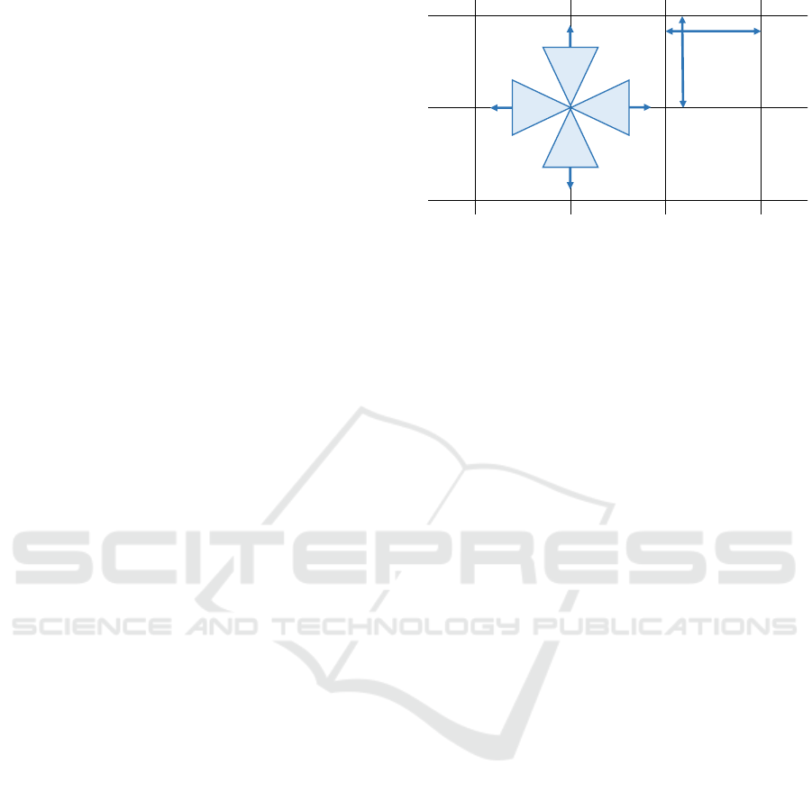
Figure 1: Images of the environments were collected fol-

lowing a grid pattern with a step size of 0.5m. For each

point of the grid, we collected four images at the four main

orientations: [0

◦

, 90

◦

, 180

◦

, 270

◦

4 EXPERIMENTAL SETTINGS

In this section, we report details about our experi-

mental setup, including the environments and how the

navigation simulations are performed, the training de-

tails of the navigation methods, and the evaluation

procedure.

4.1 Environments and Simulations

To perform experiments on both synthetic and real

environments, we follow the setup of (Zhu et al.,

2017). This setup involves running the simulations

on a grid of possible states, sampled at a regular step

of 0.5m. Each point of the grid corresponds to four

states characterized by the same position (the posi-

tion on the grid), combined with four possible orien-

tations: [0

◦

, 90

◦

, 180

◦

, 270

◦

]. For each state (position-

orientation pair), an RGB image is collected whether

from the real-world or virtual environment. Figure 1

provides a visual example of the grid pattern used to

collect the images. Each collected image represents

one discrete state in which the agent can be. The agent

can navigate through the states by performing four

possible actions: go forward, turn left, turn right, go

backward. A state-transition matrix speciﬁes which

state can be reached from another state performing

one of the actions and which states do not allow to

perform any action. A simple routine which allows

to retrieve the image observed of the next state when

taking an action at the current state is used both at

training and test time to simulate navigation. We re-

fer to the execution of one of the action in a given

state as a “step”.

For our experiments, we considered the four vir-

tual environments proposed in (Zhu et al., 2017).

Given the scarcity of datasets of real images for vi-

sual navigation (Zhu et al., 2017), we also collected

VISAPP 2020 - 15th International Conference on Computer Vision Theory and Applications

630

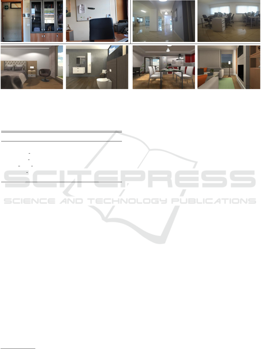
Figure 2: Sample RGB images of the real and virtual environments considered in this study. The Real Small Environment

(RSE) (top left) consists of 148 images/states. The Real Big Environment (RBE) (top right) consists of 979 images/states.

The virtual environments (bottom) have different sizes (see Table 1).

Table 1: List of the environments used to perform our ex-

periments along and related properties.

Env. name Real #states Source

RSE yes 148 this work

bathroom 02 no 180 (Zhu et al., 2017)

bedroom 04 no 408 (Zhu et al., 2017)

living room 08 no 468 (Zhu et al., 2017)

kitchen 02 no 676 (Zhu et al., 2017)

RBE yes 979 this work

images from two additional real environments for this

study. The list of all environments and their properties

is reported in Table 1. The Real Small Environment

(RSE) consists of images of a small ofﬁce, collected

with a reﬂex camera at a resolution of 5184 × 3456

pixels. The Real Big Environment (RBE) consists

of images of an open-plan ofﬁce, collected using a

robotic platform

with an on-board camera at a res-

olution of 1192 × 670 pixels. All the other environ-

ments in Table 1 have been acquired from (Zhu et al.,

2017). Sample images from the considered environ-

ments are shown in Figure 2.

4.2 Navigation Methods based on

Reinforcement Learning

Feature Extraction. We run all RL methods on fea-

tures extracted from the input images. To this pur-

pose, each RGB image has been resized to 400 × 300

pixels. The image is then processed by a ResNet-

50 CNN (He et al., 2016), pre-trained on Ima-

geNet (Deng et al., 2009) to extract its representation

vector. This has been done by removing the last clas-

We used the Sanbot Elf Robotic Platform.

http://en.sanbot.com.

siﬁcation layer from the CNN in order to obtain 2048-

dimensional representation vectors.

Training. Each of the considered models gives as

output the value of the current state and a probabil-

ity distribution over the 4 actions which can be per-

formed by the agent: go forward, turn left, turn right,

go backward. Training is performed by sampling

a number of targets proportional to the environment

size, following a uniform distribution. The second

column of Table 2 reports the number of target states

used for training on each environment. The agent is

then placed at a new random starting position and nav-

igates to the target state following the current policy.

The episode ends when the agent reaches the target

state (success) or when the maximum number of al-

lowed steps (set to 5000) is reached (fail). The tar-

get state reward was set to 20, whereas we introduce

a penalty equal to −0.1 for each navigation step or

collision. At the end of each episode, the policy is

updated to maximize the cumulative reward.

A2C - Architecture and Testing. The architecture

consists of 2 fully connected layers with 512 and 128

units respectively, Rectiﬁed Linear Units (ReLUs) as

activation functions, and an output layer with 5 units

(4 to represent a probability distribution over actions

and 1 to represent the value of the current state). Since

the method is single-target, we trained as many mod-

els as the number of targets over all environments.

This amounts to a total of 33 models. We trained all

the models for 50.000 episodes, obtaining a good con-

vergence to the optimal policy. At test time, for each

target state, we performed different navigation trials

starting from different random initial states. The third

column of Table 2 reports the number of initial states

selected per target state, for each environment.

A3C - Architecture and Testing. This method fol-

lows the architecture proposed in (Zhu et al., 2017).

A Comparison of Visual Navigation Approaches based on Localization and Reinforcement Learning in Virtual and Real Environments

631

Table 2: Number of targets seen during training and number

of test trials performed for each target. In the case of multi-

target methods, test targets are sampled at given distances

from the ones seen during training. See text for details.

Env. name # target states # test trials (x target)

RSE 3 3

bathroom 02 3 3

bedroom 04 5 5

living room 08 5 5

kitchen 02 7 7

RBE 10 10

As proposed by the authors, we feed the model with

the concatenated representations of the images of the

last 4 visited states to provide a history to the model.

The concatenated features are hence fed to a layer of

512 units. The target to reach is speciﬁed by provid-

ing also the representation of the target image as in-

put. As suggested in (Zhu et al., 2017), this input is

replicated 4 times to balance with respect to the num-

ber of history images and fed to another layer of 512

units. The 512-dimensional resulting embeddings are

concatenated and passed to the ﬁnal part of the ar-

chitecture, composed of 2 fully connected layers with

512 units each and a ﬁnal output layer with 5 units to

represent a probability distribution over actions and

the value of the current state. Since the method is

multi-target, we trained only one model for each envi-

ronment until convergence, for a total of 6 models. At

test time, to evaluate the ability of the model to gen-

eralize to unseen targets, we sampled a set of testing

targets at several distances (0, 1, 2, 4, 8 steps) from

the ones used for training. For each of the selected

testing target, we performed different navigation tri-

als starting from different random initial states. The

third column of Table 2 reports the number of initial

states selected in each trials.

4.3 Navigation Method based on

Localization

We compared the approaches based on Reinforcement

Learning with respect to a more classic navigation ap-

proach which relies on a visual localization module

based on image-retrieval. The goal of the localization

module is to determine in which state the agent is lo-

cated from the observation of the current state. Once

this information is obtained, the agent navigates to the

target by following the minimum path computed with

the Dijkstra algorithm (Cormen et al., 2001). Since

the localization algorithm may be inaccurate and fail

in some circumstances, we repeat localization and

computation of the minimum path every 5 steps, when

an invalid action is performed or when a loop in the

followed path is detected.

To perform the image-based localization, we col-

lected an additional set of images of the RBE envi-

ronment, consisting of 4072 RGB images, with a res-

olution of 1192 × 670 pixels. The images have been

acquired along random straight trajectories that cov-

ered the entire space. A 3D model of the environment

has been created using Structure From Motion (Schn-

berger and Frahm, 2016). The model has then been

aligned to a map of the environment to correct for

translation, orientation and scale. This process al-

lows to label each of the images with a 3DOF pose

which can be used for localization. Starting from this

set of images, we created a secondary regular grid

of images following the grid pattern used to acquire

the main dataset and sampling the nearest image to

each grid-point, in terms of euclidean distance and

absolute angle difference. We extracted representa-

tion vectors from each image of both the environ-

ment and the secondary set of images using a VGG-16

CNN (Simonyan and Zisserman, 2015) pre-trained on

ImageNet (Deng et al., 2009), after resizing them to

a resolution of 256 × 256 pixels and applying a cen-

ter crop, obtaining a ﬁnal size of 224 × 224 pixels.

The ﬁnal classiﬁcation layer of the CNN has been

removed to obtain 4096-dimensional representation

vectors. Given the image of the current state, the lo-

calization is performed with a nearest neighbor search

in the representations space, which allows to estimate

the state in which the actor is currently located.

4.4 Evaluation

We evaluated the performances of the different mod-

els in terms of average number of steps required to

reach the target and success rate (i.e., whether the

agent can reach the target in a limited number of

steps). All results have been obtained by averag-

ing the performance scores over all episodes obtained

starting from the randomly sampled locations. We set

a threshold of 100 steps to determine if an episode is

successful or not. We think this value is reasonable to

allow the agent to navigate without a too strict restric-

tion, but still in a limited number of steps. It is im-

portant to point out that all target and starting states

have been initially sampled and saved. All models

have been hence evaluated using the previously sam-

pled starting/target pairs for fair comparison.

VISAPP 2020 - 15th International Conference on Computer Vision Theory and Applications

632

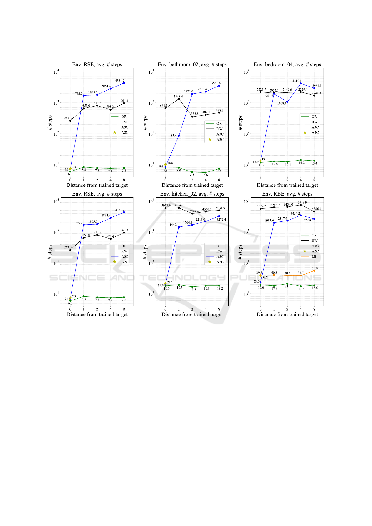
Figure 3: Performances of visual navigation methods in terms of average number of steps required to reach the target states

from random initial positions. The target states have been sampled at a distance of 0, 1, 2, 4, and 8 steps from the ones used

during training in the case of multi-target methods. This is a graphical representation of the results reported in Table 3.

5 RESULTS

Table 3 report the results of the considered visual nav-

igation methods in terms of average number of steps

and success rate required to reach the targets in the

different environments. Figure 3 further shows the

average number of steps in a visual form. The A3C

model achieves near-optimal results, comparable to

the ones obtained by the OR strong baseline on targets

seen during training (distance 0). The performances

of the A2C and A3C models on targets seen during

training (distance 0) are comparable over all environ-

ments, except for RBE. This suggests that A3C can

beneﬁt more from the additional training signal pro-

vided by larger and more complex environments. It is

worth noting tat the A3C algorithm shows a good abil-

ity to learn multiple optimal policies to different target

states of the same environment within a single model.

This is different from A2C, which can reach similar

performance on most of the environments learning a

different policy for each target. This makes A3C more

data and computation efﬁcient, requiring to train only

one model per environment, rather than one model per

target. Somewhat surprisingly, despite the good re-

sults obtained on targets seen during training, the per-

formances quickly deteriorate when the target states

A Comparison of Visual Navigation Approaches based on Localization and Reinforcement Learning in Virtual and Real Environments

633

Table 3: Performances of visual navigation methods in terms of average number of steps and success rate (in parentheses)

required to reach the target states from random initial positions. The target states have been sampled at a distance of 0, 1, 2,

4, and 8 steps from the ones used during training in the case of multi-target methods.

Env. RSE

Distance A3C A2C RW OR

0 7.1 (100) 7.3 (100) 263.3 (11) 6.0 (100)

1 1725.2 (44) - 653.0 (11) 8.3 (100)

2 1805.7 (33) - 813.8 (0) 7.8 (100)

4 2864.4 (33) - 598.2 (0) 7.6 (100)

8 4331.7 (0) - 961.3 (11) 7.8 (100)

Env. bedroom 04

Distance A3C A2C RW OR

0 12.9 (100) 13.1 2221.7 (8) 11.8 (100)

1 1961.5 (52) - 2052.1 (4) 12.8 (100)

2 1068.4 (60) - 2149.6 (12) 12.4 (100)

4 4210.1 (8) - 2229.4 (8) 14.2 (100)

8 2961.1 (4) - 1723.2 (12) 13.4 (100)

Env. kitchen 02

Distance A3C A2C RW OR

0 19.9 (100) 21.5 (100) 5912.9 (4) 18 (100)

1 1449.1 (61) - 6056 (8) 19.3 (100)

2 1704.1 (38) - 3947.4 (6) 16.8 (100)

4 2213 (22) - 4560.2 (8) 18.1 (100)

8 3272.4 (6) - 5031.9 (8) 18.2 (100)

Env. bathroom 02

Distance A3C A2C RW OR

0 8.4 (100) 10 (100) 661.1 (11) 7.8 (100)

1 85.4 (66) - 1348.4 (33) 8 (100)

2 1921 (44) - 353.8 (33) 5.8 (100)

4 2273.4 (11) - 409.1 (22) 5.6 (100)

8 3561.6 (22) - 478.3 (33) 7.4 (100)

Env. living room 02

Distance A3C A2C RW OR

0 15.8 (100) 19.2 (100) 2836 (8) 14.2 (100)

1 504.9 (64) - 3780.6 (4) 15.8 (100)

2 3950 (0) - 2766.3 (4) 15.4 (100)

4 3117.4 (28) - 3117.4 (4) 15.4 (100)

8 2563.2 20) - 4322.9 (16) 15.6 (100)

Env. RBE

Distance A3C A2C LB RW OR

0 23 (100) 36.7 (100) 39,8 (98) 5672.7 (7) 19 (100)

1 1987.6 (32) - 40.2 (95) 6246.7 (3) 17.9 (100)

2 2317.9 (15) - 38.6 (97) 6434 (3) 21.1 (100)

4 3454.2 (19) - 38.7 (96) 7549.9 (5) 17.3 (100)

8 2650.5 (32) - 55 (95) 4586.1 (7) 18.6 (100)

are sampled even at small distances from the trained

ones. These results are sub-optimal even with re-

spect to the RW baseline for smaller environments in

terms of number of steps (see Table 3 and Figure 3),

whereas marginally lower numbers of steps are re-

quired in large environments compared to RW. Nev-

ertheless, when the models are evaluated in terms of

success rate, A3C is consistently worse than RW in-

dependently from the type/size of environment. This

suggests that 1) the multi-target A3C model needs to

see large amounts of data in order to even partially

generalize to unseen targets and, 2) it is more prone

to learn a limited number of navigation policies re-

lated to the targets seen during training, rather than

a generalized policy useful for navigating to unseen

targets. Moreover, we noticed that the model hardly

converged to optimal trajectories when trained on a

number of targets greater than 10, implying a limited

ability of the training procedure to scale to a larger

number of targets/policies. In addition, the success

rate of A3C on the larger environment report an aver-

age value lower than 0.4 for targets at a distance of 1

step. The results suggest that more efforts should be

devoted to designing RL models able to learn a better

state representation space, in order to have a consis-

tent neighbourhood relationship between near states,

to efﬁciently transfer the learnt knowledge to previous

unseen samples.

We ﬁnally compare the approaches based on re-

inforcement learning with the baseline relying on vi-

sual localization (LB) on RBE. As can be assessed

from Figure 3 and Table 3, LB achieves performances

comparable to A2C and suboptimal with respect to

the ones obtained by A3C when the targets are the

ones seen during the training of the RL methods. No-

tably, while the performances of A3C quickly deteri-

orate for targets not seen during training, the perfor-

mances of LB remain overall constant. This is due to

the fact that, since the policy is not explicitly learned

in the case of LB, the method does not suffer from

over-ﬁtting to a speciﬁc target. Additionally, when

evaluated in terms of success rate, the LB approach

achieves results close to 100% and comparable to the

ones obtained by the OR baseline. While such advan-

tages over RL approaches are obtained at the expenses

of building a visual localization system, it should be

noted that methods based on localization can achieve

good results even in the presence of poor localization.

Indeed, the visual localization method of LB achieved

an average localization error of 3.86m and an average

orientation error of 53.85

◦

. The complementarity of

the results obtained by methods based on reinforce-

ment learning and the baseline relying on visual lo-

calization suggest that better results, especially for the

multi-target case, can be obtained from the integra-

tion of the two approaches. For instance, RL meth-

ods could beneﬁt from a coarse localization obtained

using simple techniques such as image-retrieval. We

leave the investigation of such integration to future

works.

VISAPP 2020 - 15th International Conference on Computer Vision Theory and Applications

634

6 CONCLUSION

In this paper, we compared visual navigation methods

based on reinforcement learning and localization. We

performed experiments on differently sized discrete-

state environments composed of both virtual and real

images. The results suggest that, despite the avail-

ability of multi-target approaches, visual navigation

methods based on reinforcement learning have difﬁ-

culties to generalize to targets unseen during training.

On the contrary, a simple baseline which relies on in-

accurate localization achieves similar results on tar-

gets seen during training and generalizes better to un-

seen targets. These observations suggest that methods

based on reinforcement learning could beneﬁt even

from inaccurate localization. Future works can inves-

tigate approaches to fuse visual navigation methods

based on reinforcement learning and localization.

ACKNOWLEDGEMENTS

This research is supported by OrangeDev s.r.l. and

Piano della Ricerca 2016-2018, Linea di Intervento 2

of DMI, University of Catania.

REFERENCES

Arandjelovic, R., Gronat, P., Torii, A., Pajdla, T., and Sivic,

J. (2016). Netvlad: Cnn architecture for weakly super-

vised place recognition. In CVPR, pages 5297–5307.

Bojarski, M., Testa, D. D., Dworakowski, D., Firner, B.,

Flepp, B., Goyal, P., Jackel, L. D., Monfort, M.,

Muller, U., Zhang, J., Zhang, X., Zhao, J., and Zieba,

K. (2016). End to end learning for self-driving cars.

CoRR, abs/1604.07316.

Cormen, T. H., Stein, C., Rivest, R. L., and Leiserson, C. E.

(2001). Introduction to Algorithms. McGraw-Hill

Higher Education, 2nd edition.

Deng, J., Dong, W., Socher, R., Li, L.-J., Li, K., and Fei-

Fei, L. (2009). ImageNet: A Large-Scale Hierarchical

Image Database. In CVPR.

Giusti, A., Guzzi, J., Cires¸an, D. C., He, F.-L., Rodr

ıguez,

J. P., Fontana, F., Faessler, M., Forster, C., Schmidhu-

ber, J., Di Caro, G., et al. (2015). A machine learning

approach to visual perception of forest trails for mo-

bile robots. RA-L, 1(2):661–667.

Gupta, S., Davidson, J., Levine, S., Sukthankar, R., and Ma-

lik, J. (2017). Cognitive mapping and planning for

visual navigation. In CVPR, pages 7272–7281.

He, K., Zhang, X., Ren, S., and Sun, J. (2016). Deep resid-

ual learning for image recognition. In CVPR, pages

770–778.

Hong Zhang and Ostrowski, J. P. (2002). Visual motion

planning for mobile robots. T-RA, 18(2):199–208.

egou, H., Douze, M., Schmid, C., and P

erez, P. (2010).

Aggregating local descriptors into a compact image

representation. In CVPR, pages 3304–3311.

Kempka, M., Wydmuch, M., Runc, G., Toczek, J., and

skowski, W. (2016). Vizdoom: A doom-based ai re-

search platform for visual reinforcement learning. In

CIG, pages 1–8.

Kendall, A., Grimes, M., and Cipolla, R. (2015). Posenet:

A convolutional network for real-time 6-dof camera

relocalization. In ICCV, pages 2938–2946.

Konda, V. R. and Tsitsiklis, J. N. (2000). Actor-critic algo-

rithms. In NIPS, pages 1008–1014.

Mirowski, P., Pascanu, R., Viola, F., Soyer, H., Ballard,

A. J., Banino, A., Denil, M., Goroshin, R., Sifre,

L., Kavukcuoglu, K., Kumaran, D., and Hadsell, R.

(2016). Learning to navigate in complex environ-

ments. CoRR, abs/1611.03673.

Mnih, V., Badia, A. P., Mirza, M., Graves, A., Lillicrap, T.,

Harley, T., Silver, D., and Kavukcuoglu, K. (2016).

Asynchronous methods for deep reinforcement learn-

ing. In ICML, pages 1928–1937.

Mnih, V., Kavukcuoglu, K., Silver, D., Graves, A.,

Antonoglou, I., Wierstra, D., and Riedmiller, M.

(2013). Playing atari with deep reinforcement learn-

ing. In NIPS Deep Learning Workshop.

Orlando, S. O., Furnari, A., Battiato, S., and Farinella,

G. M. (2019). Image-based localization with simu-

lated egocentric navigations. In VISAPP.

Ragusa, F., Furnari, A., Battiato, S., Signorello, G., and

Farinella, G. (2019). Egocentric visitors localization

in cultural sites. JOCCH, 12:1–19.

Ross, S., Gordon, G., and Bagnell, J. (2010). A reduction

of imitation learning and structured prediction to no-

regret online learning. JMLR, 15.

Sattler, T., Leibe, B., and Kobbelt, L. (2016). Efﬁcient &

effective prioritized matching for large-scale image-

based localization. PAMI, 39(9):1744–1756.

Savva, M., Kadian, A., Maksymets, O., Zhao, Y., Wijmans,

E., Jain, B., Straub, J., Liu, J., Koltun, V., Malik, J.,

et al. (2019). Habitat: A platform for embodied ai

research. arXiv preprint arXiv:1904.01201.

Schnberger, J. L. and Frahm, J. (2016). Structure-from-

motion revisited. In CVPR, pages 4104–4113.

Simonyan, K. and Zisserman, A. (2015). Very deep convo-

lutional networks for large-scale image recognition. In

ICLR.

Thrun, S., Burgard, W., and Fox, D. (2005). Probabilistic

robotics. MIT press.

Ulrich, I. and Borenstein, J. (1998). Vfh+: Reliable obstacle

avoidance for fast mobile robots. In ICRA, volume 2,

pages 1572–1577.

Xia, F., Zamir, A. R., He, Z., Sax, A., Malik, J., and

Savarese, S. (2018). Gibson env: Real-world percep-

tion for embodied agents. In CVPR, pages 9068–9079.

Zhu, Y., Mottaghi, R., Kolve, E., Lim, J. J., Gupta, A., Fei-

Fei, L., and Farhadi, A. (2017). Target-driven visual

navigation in indoor scenes using deep reinforcement

learning. In ICRA, pages 3357–3364.

A Comparison of Visual Navigation Approaches based on Localization and Reinforcement Learning in Virtual and Real Environments

635