Visual Exploration of 3D Shape Databases Via Feature Selection

Xingyu Chen

1,2 a

, Guangping Zeng

1 b

, Ji

ı Kosinka

2 c

and Alexandru Telea

3 d

School of Computer and Communication Engineering, University Science and Technology Beijing, Beijing, China

Bernoulli Institute, Faculty of Science and Engineering, University of Groningen, The Netherlands

Utrecht University, The Netherlands

Keywords:

Content-based Shape Retrieval, Multidimensional Projections, Feature Selection, Visual Analytics.

Abstract:

We present a visual analytics approach for constructing effective visual representations of 3D shape databases

as projections of multidimensional feature vectors extracted from their shapes. We present several methods

to construct effective projections in which different-class shapes are well separated from each other. First,

we propose a greedy heuristic for searching for near-optimal projections in the space of feature combina-

tions. Next, we show how human insight can improve the quality of the constructed projections by iteratively

identifying and selecting a small subset features that are responsible for characterizing different classes. Our

methods allow users to construct high-quality projections with low effort, to explain these projections in terms

of the contribution of different features, and to identify both useful features and features that work adversely

for the separation task. We demonstrate our approach on a real-world 3D shape database.

1 INTRODUCTION

Recent developments in 3D content creation and 3D

content acquisition technologies, including modeling

and authoring tools and 3D scanning techniques, have

led to a rapid increase in the number and complex-

ity of available 3D models. Such models are typi-

cally stored in so-called shape databases (ShapeNet,

2019; ITI DB, 2019). Such databases offer next var-

ious mechanisms enabling users to browse or search

them to locate models of interest for a speciﬁc appli-

cation at hand.

As shape databases increase, so does the difﬁ-

culty that users have in locating models of inter-

est therein (Tangelder and Veltkamp, 2008). Typi-

cal mechanisms offered to support this task include

searching by keywords, browsing the database along

one or a few predeﬁned hierarchies, or content-based

shape retrieval (CBSR). While efﬁcient for certain

scenarios, all these mechanisms have limitations:

Keyword search assumes a good-quality labeling of

shapes with relevant keywords, and also that the user

is familiar with relevant search terms. Hierarchy

browsing is most effective when the organization of

https://orcid.org/0000-0002-3770-4357

https://orcid.org/0000-0003-0494-3877

https://orcid.org/0000-0002-8859-2586

https://orcid.org/0000-0003-0750-0502

shapes follows the way the user wants to explore

them. Finally, CBSR works well when the user aims

to search for shapes similar to an existing query shape.

Besides the above targeted use-cases, more

generic ones involve users who simply want to ex-

plore the entire database to see what it contains. This

is relevant in cases where users want to ﬁrst get a good

overview of what a database contains before deciding

to invest more effort into exploring or using it; and

also in cases where users do not have speciﬁc searches

in mind. Existing mechanisms offered for the above

scenarios are linear in nature, showing either a small

part of the database at a single time and/or asking the

user to perform lengthy navigations to create a mental

map of the database itself, much like when navigating

a web domain.

We address this task by a different, visual, ap-

proach. We construct a compact and scalable

overview of an entire shape database, with shapes or-

ganized by similarity. We offer details-on-demand

mechanisms to enable users to control the separa-

tion quality of the similar-shape groups in the visual

overview; understand what makes a set of shapes sim-

ilar (or two or more sets of shapes different); and ﬁnd

features that have high, respectively little, value for

the shape classiﬁcation task. Our approach is sim-

ple to use; requires no prior knowledge of the orga-

nization of a shape database; nor a prior organization

Chen, X., Zeng, G., Kosinka, J. and Telea, A.

Visual Exploration of 3D Shape Databases Via Feature Selection.

DOI: 10.5220/0008950700420053

In Proceedings of the 15th Inter national Joint Conference on Computer Vision, Imaging and Computer Graphics Theory and Applications (VISIGRAPP 2020) - Volume 3: IVAPP, pages 42-53

ISBN: 978-989-758-402-2; ISSN: 2184-4321

or labeling of the database; handles any type of 3D

shape represented by a polygon mesh; and scales vi-

sually and computationally to real-world large shape

databases. Additionally, our proposal is useful for

both end users (who aim to explore a shape database)

and technical users (who aim to engineer features to

query or classify shapes in such databases).

This paper is structured as follows. Section 2 out-

lines related work in exploring 3D shape databases.

Section 3 details our pipeline that consists of shape

normalization, feature extraction, and dimensionality

reduction. Section 4 presents our automatic and user-

driven methods for constructing high-quality projec-

tions for exploring shape databases, and demonstrates

these on a real-world shape database. Section 6 con-

cludes the paper.

2 RELATED WORK

Searching and exploring 3D shape databases can be

structured along three modalities, as follows.

Keyword search uses words to search for shapes

whose annotation data contains those words. It

is the simplest to support, and therefore old-

est and most widespread form of search for

3D content, present in many shape databases,

such as TurboSquid (TurboSquid, Inc., 2019) and

Aim@Shape (Aim@Shape, 2019), to mention just a

few. Such databases allow providers to upload mod-

els with associated keywords for subsequent search.

However, keyword lists are only weakly structured,

possibly containing redundant or vague keywords, po-

tentially added this way to increase exposure rate.

Besides general-purpose databases of this type, more

specialized ones exist, such as containing 3D shapes

related to space exploration (NASA, 2019). Overall,

keyword search is popular and widely supported, but

works best for targeted searches performed by users

aware of a database’s organization, require a good an-

notation with speciﬁc keywords, and is less effective

for overall exploration.

Hierarchical exploration systems organize shapes

along different criteria, following an existing tax-

onomy of the targeted 3D shape universe at hand.

Such systems support exploration (apart from key-

word search) by allowing users to browse the

hierarchy, with shapes or shape categories de-

picted by thumbnails, much like when exploring

a ﬁle system. Examples of such systems are the

Princeton Shape Benchmark (Shilane et al., 2004),

Aim@Shape (Aim@Shape, 2019), or the ITI 3D

search engine (ITI DB, 2019) that allows browsing

multiple hierarchically-organized shape databases.

Hierarchy browsing supports browsing better than

keyword-based search. Yet, it typically only allows

examining a single path (shape subset) at a time, and

cannot provide a rich global overview of an entire

database. Moreover, its effectiveness relies on the

provided hierarchy, which may or may not match the

way users see the grouping of shapes.

Content Based Shape Retrieval (CBSR) allows

users to search for shapes similar to a given query

shape, and therefore depend far less on an upfront or-

ganization of the database in terms of suitable key-

words or hierarchies and/or on the user’s familiar-

ity with these. Good surveys of CBSR methods

are provided by (Bustos et al., 2005; Tangelder and

Veltkamp, 2008). These methods essentially extract

a high-dimensional descriptor from the query and

database shapes, and then search and retrieve the most

similar shapes to the query based on a suitable dis-

tance metric in descriptor space. Many types of de-

scriptors and distance metrics have been proposed, as

follows. Global descriptors, such as shape elongation,

eccentricity, and compactness, are simple, yet crude

ways to discriminate between highly different shapes.

Local descriptors, such as saliency, shape thickness,

and shape contexts capture more ﬁne-grained shape

details (Shtrom et al., 2013; Rusu et al., 2009; Shapira

et al., 2008; Tasse et al., 2015). Topological descrip-

tors, such as based on curve skeletons (Jalba et al.,

2012) or surface skeletons (Feng et al., 2016) cap-

ture the part-whole shape structure. Finally, view-

based descriptors capture the appearance of the shape

from multiple viewpoints (Cyr and Kimia, 2001; Shen

et al., 2003). Kalogerakis et al. (Kalogerakis et al.,

2010) provide a tool to compute several types of shape

features. Apart from such hand-engineered descrip-

tors, deep learning has proved effective in automat-

ically extracting low-dimensional representations of

shape with high accuracy for query tasks (Su et al.,

2015). CBSR frees the user from the burden of speci-

fying keywords or choosing explicit navigation paths

in a hierarchy to examine a shape database. Addition-

ally, CBSR assists in ﬁnding the most similar shapes

to a given prototype (query). However, CBSR does

not readily support the task of general-purpose explo-

ration of a shape database, e.g., seeing how all the

shapes within it are organized in terms of similarity.

Summarizing the above, keyword search, hierar-

chical exploration, and CBSR offer largely comple-

mentary mechanisms for exploring a shape database,

and can be readily combined in a 3D database ex-

ploration system. However, as outlined, none of

these methods offer a compact, complete, and detailed

overview of an entire database. Moreover, such mech-

anisms do not explain why a set of shapes are deemed

Visual Exploration of 3D Shape Databases Via Feature Selection

similar. In earlier work, Rauber et al. (Rauber et al.,

2015) have used interactive feature selection to im-

prove image classiﬁcation, which is related, but not

the same, to our goal of exploring data collections.

Such functionalities are essential in contexts where

users do not know precisely what they are looking

for, and would like to understand the information con-

tained in a database before proceeding to more spe-

ciﬁc queries.

3 PROPOSED METHOD

To support the overall exploration of 3D shape

databases, we propose to augment existing mecha-

nisms (keyword search, hierarchies, and CBSR) by

a visual navigation approach. Our approach allows

users to see a complete overview of an entire database

and the way shapes are organized within in terms of

similarity. Next, it allows selecting speciﬁc shapes

or shape properties and ﬁnding similar shapes (from

the perspective of one or several such properties), and

also ﬁnding out how properties discriminate between

different shapes. We now detail our approach.

3.1 Overview

We start by introducing some notations. A mesh

m = (V = {x

}, F = { f

}) is a collection of vertices

⊂ R

and faces f

, assumed to be triangles for sim-

plicity. A shape database is a set of shapes M = {m

No restrictions are placed here, i.e., shapes can be of

different kinds, sampling resolutions, and require no

extra organization or annotations, e.g., classes or hi-

erarchies.

Our key idea is to present a visual overview

of M in which every shape m

is represented by

a thumbnail rendering thereof, and visual distances

between two shapes m

and m

reﬂect their simi-

larity. The visual overview is interactively linked

with detail views in which users can explore spe-

ciﬁc shape details. The combination of overview and

details, following Shneiderman’s visual exploration

mantra (Shneiderman, 1996), enables both free and

targeted exploration of the shape database along the

use-cases outlined in Sec. 2.

We create our overview-and-detail visual explo-

ration as follows. First, we preprocess all meshes

in M so as to normalize them in terms of sampling

resolution and size. Secondly, we extract local fea-

tures from all meshes m ∈ M (Sec. 3.3). These fea-

tures capture the respective shapes at a ﬁne level of

detail. Next, we aggregate local features into ﬁxed-

length feature vectors (Sec. 3.4). Finally, we use

a dimensionality-reduction algorithm to project the

shapes, represented by their feature vectors, onto 2D

screen space (Sec. 3.5). We describe all these steps

next.

3.2 Preprocessing

Since we do not pose any constraint on the shapes in

M, these can come with virtually any sampling reso-

lution, orientation, and at any scale. Such variations

are known to pose problems when computing virtu-

ally any type of shape descriptor (Bustos et al., 2005).

Hence, as a ﬁrst step, we normalize all shapes m ∈ M

by ﬁrst remeshing them, with a target edge-length of

1% of m’s bounding-box diagonal. Next, we translate

and scale the remeshed shapes to ﬁt the [−1, 1]

cube.

3.3 Local Feature Extraction

To characterize shapes, we extract several so-called

local features from each. Such features describe the

shape at or in the neighborhood of every vertex x

∈ m

and are therefore good at capturing local characteris-

tics. We compute seven local feature types, as fol-

lows.

Gaussian Curvature (Gc): Gaussian curvature de-

scribes the overall ﬂatness of a shape close to a given

point. For every vertex x ∈ m we compute its Gaus-

sian curvature as

Gc(x) = 2π −

∑

f ∈F(x)

x, f

, (1)

where F(x) is the set of faces in F incident with x and

x, f

is the angle in face f at vertex x.

Average Geodesic Distance (Agd): We estimate the

geodesic distance d(x, y) between a pair of vertices

x and y of m as the geometric length of the short-

est path in the edge connectivity graph of m be-

tween x and y. This distance can be easily and ef-

ﬁciently estimated using Dijkstra’s shortest-path al-

gorithm with A* heuristics and edge weights equal

to edge lengths. More accurate estimations of the

geodesic distance between two points on a polygonal

mesh exist, including computing the distance ﬁeld (or

transform) DT (x) of x over F and tracing a stream-

line in −∇DT (x) from x until it reaches y (Peyre and

Cohen, 2005); GPU minimization of cut-length using

pivoting slice planes passing through x and y (Jalba

et al., 2013); or hybrid search techniques (Verma and

Snoeyink, 2009). While more accurate than the Di-

jkstra approach we use, these methods are consid-

erably more complex to implement, slower to run,

and require careful tuning and/or specialized plat-

forms (GPU support). For a detailed comparison of

IVAPP 2020 - 11th International Conference on Information Visualization Theory and Applications

geodesic estimation methods on polygonal meshes,

we refer to (Jalba et al., 2013). More importantly, we

do not use the individual geodesic lengths, but aggre-

gate them into per-shape feature vectors (Sec. 3.4). As

such, high geodesic estimation precision is less im-

portant.

Given the above, we estimate the average geodesic

distance of a vertex x as

Agd(x) =

∑

y∈V

d(x, y)

|V |

. (2)

Normal Diameter (Nd): We ﬁrst estimate the surface

normal at a vertex x as

n(x) =

∑

f ∈F(x)

n( f )θ

x, f

, (3)

where n( f ) is the outward normal of face f . Given

the above, let r be a ray starting at x and advancing

in the direction −n(x). The normal diameter Nd(x)

is then the distance along r from x to the closest face

f ∈ F \F(x).

Normal Angle (Na) and Point Angle (Pa): These

features describe how vertices x ∈ V are spread

around the shape itself. In detail, let e

be the domi-

nant eigenvector of the shape covariance matrix given

by all vertices V . As known, e

gives the direction

in which the shape spreads the most. Next, for every

vertex x ∈ V , we deﬁne the normal angle Na(x) as the

angle (dot product) between e

and the surface nor-

mal n(x); and the Point Angle Pa(x) as the angle (dot

product) between e

and the vector c − x, where c is

the barycenter of m.

Shape Context (Sc): The shape context descriptor

is a 2D histogram that characterizes how vertices of

a shape are ‘seen’ in terms of distance and orienta-

tion from a given vertex of that shape (Belongie et al.,

2001). For a vertex x ∈ V , the shape context de-

scribes the number of vertices in V that are within

a given distance range and direction range to x. To

compute Sc, we ﬁrst build a local coordinate system

at every vertex x, using the eigenvectors of the shape

covariance matrix in the neighborhood of x. This

ensures that this coordinate system is aligned with

the shape locally — one of its axes will be the nor-

mal n(x), whereas the two other ones are tangent to

the surface of m at x. Next, we discretize the ori-

entations around x into the eight octants of the local

coordinate system, and distances using a set of bins

(distance ranges) (t

i+1

) deﬁned by a distance-set

T = {0, t

, . . . , t

, 1}, n ∈ N

. In practice, we use

T = [0, 0.1, 0.3, 1]. Hence, for each vertex x, we get a

shape context vector with 8 × 3 = 24 elements.

Point Feature Histogram (PFH): PFH (Rusu et al.,

2009) is a complex descriptor that captures the local

geometry in the vicinity of a vertex. Given a pair of

u = m

v = (

y − y) × u

w = u × v

y − y

Figure 1: PFH descriptor computation (Shtrom et al., 2013).

vertices y and

y, one ﬁrst deﬁnes a local coordinate

frame (u, v, w) as

u = m,

v = (

y − y) × u,

w = u × v,

(4)

where m is the vertex normal at y (Fig. 1). Next, the

variation of the shape geometry between points y and

y is captured by three polar coordinates

α = v ·

φ = u ·

y − y

y − yk

θ = arctan2(w ·

m, u ·

m),

(5)

where

m is the vertex normal at

y. Next, three

histograms are built to capture the distributions of

α, φ, θ for a given vertex x by considering all pairs

(y,

y) ∈ N

x,k

× N

x,k

in the k-nearest neighbors N

x,k

of x. In practice, we set k = 30 and use 5 bins for

each histogram. This delivers a PFH feature vector of

= 125 entries.

Fast Point Feature Histogram (FPFH): While PFH

models a neighborhood N

x,k

by all its point-pairs, the

Simpliﬁed Point Feature Histogram (SPFH) models

x,k

by the characteristics of the pairs (x, y ∈ N

x,k

We proceed analogously to binning the α, φ, θ distri-

butions in three histograms of 11 bins each, obtain-

ing a feature vector of 3 × 11 = 33 elements. With

this vector, we ﬁnally compute the FPFH value of a

vertex x following (Rusu et al., 2009) as the distance-

weighted average of the SPFH values over the neigh-

borhood N

x,k

FPFH(x) = SPFH(x) +

∑

y∈N

x,k

SPFH(y)

kx − yk

. (6)

3.4 Feature Vector Computation

The features described in Sec. 3.3 are local, i.e., they

take different values for every mesh vertex x ∈ V . To

be able to compare meshes to each other, we need to

reduce these to same-length global descriptors. For

this, we use a simple histogram-based solution that

aggregates the values of every local descriptor, at all

Visual Exploration of 3D Shape Databases Via Feature Selection

vertices of a mesh, into a ﬁxed-length (10 bin) his-

togram. Note that some descriptors are by deﬁnition

high-dimensional — for instance, the shape context

Sc has 24 dimensions. Hence, for a d-dimensional

descriptor, we compute a histogram having 10d bins.

Table 1 shows the local features, their dimensional-

ity, and the number of bins used to quantize each.

Summarizing, we reduce every shape m to a 1870-

dimensional feature vector F .

3.5 Dimensionality Reduction

So far, we have reduced a shape database M to a

set of |M| 1870-dimensional feature vectors. We

next create a visual representation of the shape

database by projecting all these vectors onto 2D us-

ing the well-known t-SNE dimensionality reduction

method (van der Maaten and Hinton, 2008). Sim-

ply put, t-SNE constructs a 2D scatterplot P(M) =

{P(m

)}, where every shape m

∈ M is represented

by a point P(m) ∈ R

, so that the distances between

scatterplot points reﬂect (encode) the similarities of

their feature vectors.

An important concern when proposing such a rep-

resentation is to gauge its quality. To do this, we

use the classes (labels) of the shapes. For a database

where each shape m has a categorical label c(m) ∈ C,

where C is a set of categories (e.g., keywords describ-

ing the different shapes in a database), we deﬁne the

neighborhood hit NH(m) as the proportion of the k-

nearest neighbors of P(m) that have the same label

c(m) as m itself (Paulovich et al., 2008). In prac-

tice, we set k = 10, following related applications

that gauge projection quality (Paulovich et al., 2008).

With this, we can next deﬁne the neighborhood hit of

an entire class c ∈ C as

∑

m∈M:c(m)=c

NH(m)

|m ∈ M : c(m) = c|

. (7)

Finally, at the highest aggregation level, we deﬁne the

neighborhood hit for an entire scatterplot P(M) for a

Table 1: Local features, their dimensionalities and binning.

Name Dimensionality Bins

Gaussian curvature (Gc) 1 10

Average geodesic distance (Agd) 1 10

Normal diameter (Nd) 1 10

Normal angle (Na) 1 10

Point angle (Pa) 1 10

Shape context (Sc) 24 240

Point Feature Histogram (PFH) 125 1250

Fast Point Feature Histogram (FPFH) 33 330

Total 1870

shape database M as

(M) =

∑

m∈M

NH(m)

|M|

. (8)

The above two NH metrics describe how a mesh

(point in the 2D projection scatterplot) is separated

from points of different kinds: NH

shows whether

a group of points representing same-class meshes is

well separated in a scatterplot (something we desire

since we want next to use the scatterplot to answer the

question “How many shape classes are in a database,

and how similar are they to each other?”). NH

shows

how well a whole scatterplot can represent an entire

shape database. Both NH metrics range between 0

and 1, with higher values indicating better separation,

which is preferred.

4 APPLICATIONS

We next demonstrate our visual exploration ap-

proach on a subset of the Princeton Shape Bench-

mark (Shilane et al., 2004) having 280 meshes from

14 classes, with 20 meshes from each class. As out-

lined earlier, these meshes are not labeled, hierarchi-

cally organized, or otherwise preprocessed.

4.1 Optimal Scatterplot Creation

The projection scatterplot (Sec. 3.5) is the central

view that shows an entire shape database. Hence,

creating a good scatterplot is important for all explo-

ration tasks addressed next. In this section, we ex-

plore the following questions:

Q1: How can we create a good projection scatterplot?

Q2: Which features are best for grouping simi-

lar shapes (and, conversely, separating different

shapes) in the scatterplot?

Q3: Which is the minimal set of features required to

generate a good-quality scatterplot?

Concerning Q1, we could directly create and

examine a t-SNE projection of the whole shape

database as encoded by the 1870-dimensional fea-

ture vectors we extracted (Sec. 3.4). However, us-

ing t-SNE is not always easy, especially for high-

dimensional data: This method maps similarities (of

feature vectors) non-linearly to 2D distances; also,

tuning t-SNE’s parameters to yield a good embed-

ding of high-dimensional feature vectors is notori-

ously hard (Wattenberg, 2016). Hence, we ﬁrst ex-

plore the simpler solution of projecting only subsets

of all extracted features. As we have 8 feature types

(Tab. 1), a natural idea is to try all combinations of

IVAPP 2020 - 11th International Conference on Information Visualization Theory and Applications

NH value highlow

features: Gc, Na, Pa, Agd, PFH NH

: 0.859

plier: 1.0

teddy: 0.985

cup: 0.98

ant: 0.975

fish: 0.945

chair: 0.895

glasses: 0.88

airplane: 0.875

table: 0.87

human: 0.855

hand: 0.805

fourleg: 0.765

bird: 0.66

octopus: 0.53

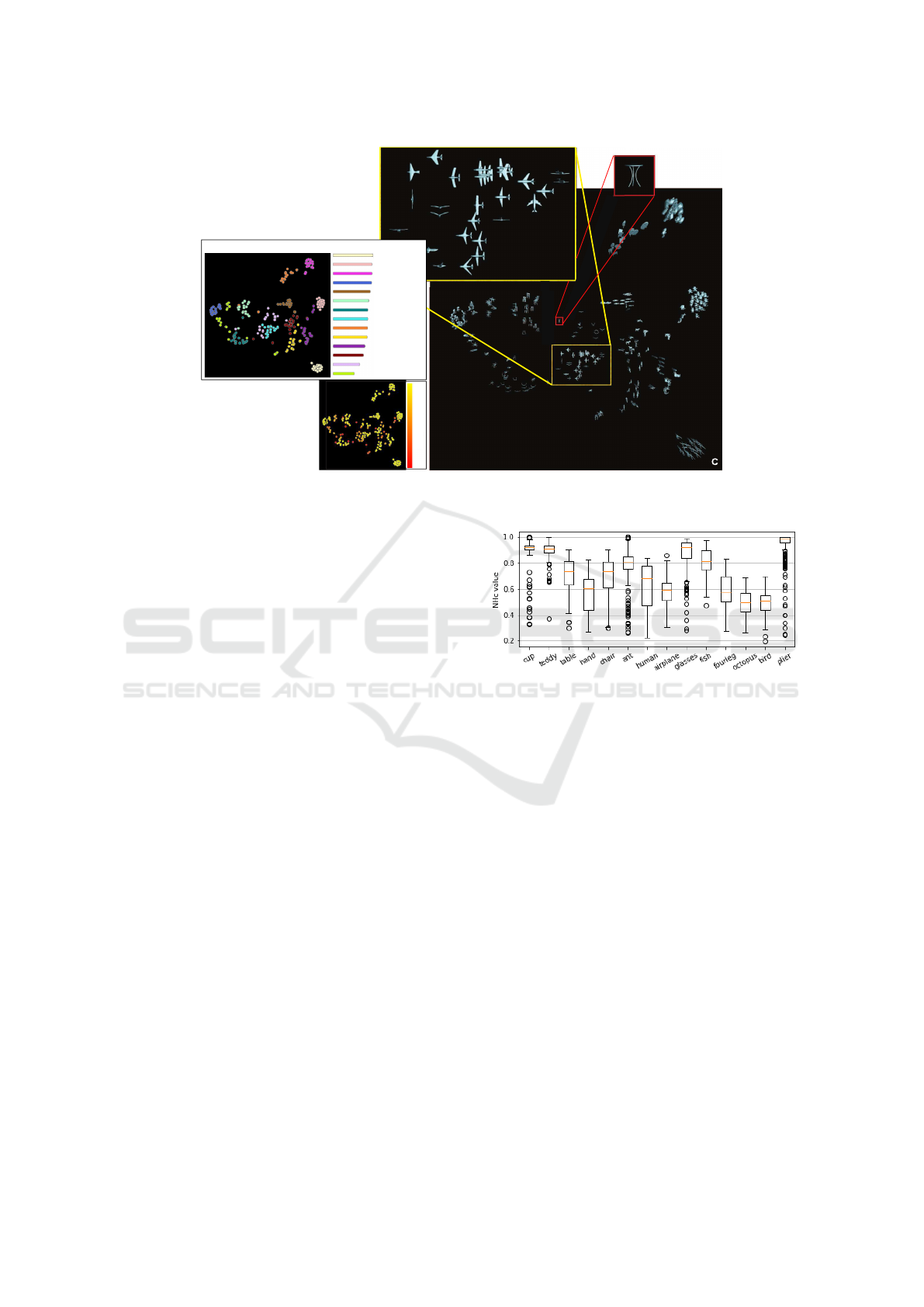
Figure 2: Three views of the optimal projection scatterplot for the Princeton Shape Database, depicting classes and their NH

values and the overall plot quality NH

(A), per-shape NH values (B), and actual shape thumbnails (C).

groups of feature types. This yields 2

−1 = 255 pos-

sible projection scatterplots. Following the scagnos-

tics idea (Tukey and Tukey, 1988; Wilkinson et al.,

2006), we compute all these scatterplots (using t-

SNE) and select the one having the highest quality,

measured by its NH

value.

Figure 2 shows three views of the optimal projec-

tion scatterplot, as follows. Image A shows the scat-

terplot with points (shapes m ∈ M) colored by their

class value c(m). The text atop this image indicates

the feature subset leading to this optimal scatterplot

(highest NH

= 0.859 value), namely (Gc, Na, Pa,

Agd, PFH). The bar chart in image A shows the NH

values for all classes, with high values (well sepa-

rated classes) at the top. From this, we can see that

pliers are perfectly separated from all other classes

(NH

pliers

= 1), while octopus is least well separated

(NH

octopus

= 0.53). Image B shows the optimal scat-

terplot colored by NH values for all shapes, ranging

between red (low NH) to yellow (high NH). Red

points in this image show shapes which are not pro-

jected well — that is, placed close to shapes having

different classes. Finally, image C shows the opti-

mal scatterplot with shapes depicted by thumbnails.

From this image, we ﬁnd that shapes of the classes pli-

ers, teddies, cups, ants, and ﬁshes are well projected.

However, birds are mixed with airplanes; and fourlegs

are mixed with humans and hands. The octopus class

is visually split in the projection into several parts.

While this optimal scatterplot is not perfect, it is still

formally the best one we can create given the combi-

nations of our 8 available features. Indeed, while class

separation is not perfect, closely-projected shapes are

Figure 3: NH

statistics for the 14 classes in the shape

database for all considered 255 projection scatterplots.

still quite similar. For instance, ants are surrounded by

octopuses, which is arguably logical, since both shape

types have many thin and spread legs. Similarly, air-

planes and birds are close to each other; indeed, both

have wings and are relatively ﬂat.

Figure 3 shows boxplot statistics of the NH

val-

ues for the 14 shape classes in our database for the

255 created projection scatterplots. Ideally, we would

like to see that every class has a very high NH

value.

However, we see that birds and octopuses have quite

low NH

values, conﬁrming the insights obtained ear-

lier by visually examining the projection (Fig. 2).

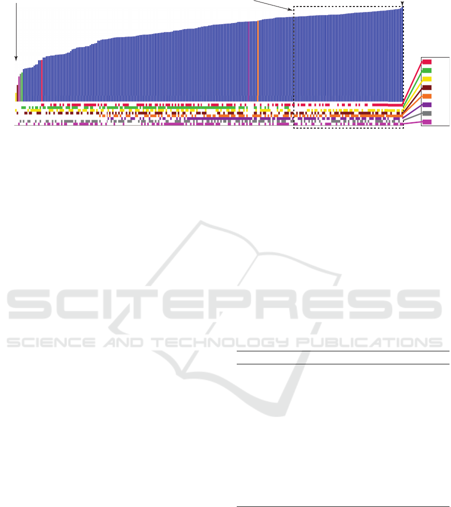
Finally, Fig. 4 shows a complete view of how fea-

tures affect the quality of the produced projections.

The bar chart shows the NH

values of all possible

255 projections created by combining our 8 features

types, sorted in increasing values from left to right.

The matrix plot below the bar chart shows which fea-

tures (color coded according to the legend at the right)

are used by which projection. Projections using more

than one feature have blue bars; projections that use

exactly one feature have their bars colored by the re-

Visual Exploration of 3D Shape Databases Via Feature Selection

PFH

FPFH

Agd

0.83

0.0

Feature

Legend

best projectionworst projection

top 30% best projections

Figure 4: A bar chart showing the NH

scores of 255 projections, sorted on increasing value (best projections to the right,

worst ones to the left). The color blocks under a bar show which features are used for that projection (the feature color legend

on the right). Bars which are not blue only use one feature, whose identity colors the bar. Scanning the color matrix below the

bars row-wise tells us which projections use which features. We see that PFH (orange) and FPFH (purple) are good features

since their blocks are close to the right. Conversely, Sc (green) is not a very useful feature since its blocks are spread to the

left.

spective feature. This plot gives us several insights:

(1) The quality difference between the best and worst

projections is signiﬁcant (NH

0.831 vs 0.38), with

better projections using more features than poor ones;

(2) some features are really instrumental in achieving

high quality, e.g. PFH (orange) and FPFH (purple),

which appear consistently in the right of the matrix

plot in Fig. 4, whereas other features are actually ad-

versely affecting quality, e.g. Sc (green) which ap-

pears in the left of the matrix plot. This indicates ei-

ther that Sc is not a useful feature for discriminating

classes in this database or that it is poorly evaluated,

e.g., by an insufﬁciently dense sampling. (3) Over-

all, the right of the matrix is more full than its left

part, which means that using more features produces

better segregating projections, although the relation

is not monotonic. (4) The highest-quality projections

(roughly, rightmost third of the bar chart) consistently

use the same mix of features (Gc, Na, Pa, PFH, FPFH,

Agd, Nd). (5) The patterns in the matrix plot of dif-

ferent features look different, which means there are

no redundant features in the considered set.

4.2 Fast Computation of Near-optimal

Projection Scatterplot

Computing all possible scatterplots given a feature

vector F to ﬁnd the optimal one is expensive, espe-

cially when the set F is large. We next propose a

greedy algorithm to accelerate this task (Alg. 1). The

parameter s gives the maximum size of the feature-set

to search for. For every search iteration,



|F |



fea-

ture combinations are examined, and the best one, in

terms of the realized NH

value, is retained. Better so-

lutions are obtained for larger s values, at the expense

of longer search times. When s = |F |, Alg. 1 com-

pares all possible 2

|F |

feature combinations. From

our tests, a quite good solution in terms of NH

value

can be found by setting s = 1. For this setting, the

time complexity of our algorithm is O(|F |

Table 2 shows the results of our greedy algorithm,

executed 5 times, to account for the stochastic nature

of the t-SNE projection. For every round, we indi-

cate the time taken by exhaustive search vs our greedy

search, and also the number of t-SNE projections be-

ing evaluated. We see that our algorithm yields prac-

tically the same NH

quality as the exhaustive search,

but is roughly 5 times faster.

Algorithm 1: Computing near-optimal feature sets.

Input: Set of features F ; maximal size s, 1 ≤ s ≤ |F |, of

feature-set to search for,

Output: Near-optimal feature set C,

1: C := ø, C

new

:= ø;

2: repeat

3: C := C

new

4: for each F

sub

⊆ F , |F

sub

| ≤ s do

5: C

temp

:= (C ∪ F

sub

) − (C ∩ F

sub

)

6: if NH

temp

) > NH

new

) then

7: C

new

:= C

temp

;

8: end if

9: end for

10: until (C

new

= C );

11: return C ;

4.3 User-driven Projection Engineering

Section 4.2 showed how we can automatically se-

lect features from the eight existing feature classes

(Tab. 1) to create a projection scatterplot which best

separates shapes from different classes. However, us-

ing this automatic approach has some disadvantages:

(1) It is expensive, even when using the proposed

IVAPP 2020 - 11th International Conference on Information Visualization Theory and Applications

1. model and feature selector

2. original scatterplot

6. separation

control

selected features

4. scoring

methods

5. refined scatterplot

3. feature scoring view

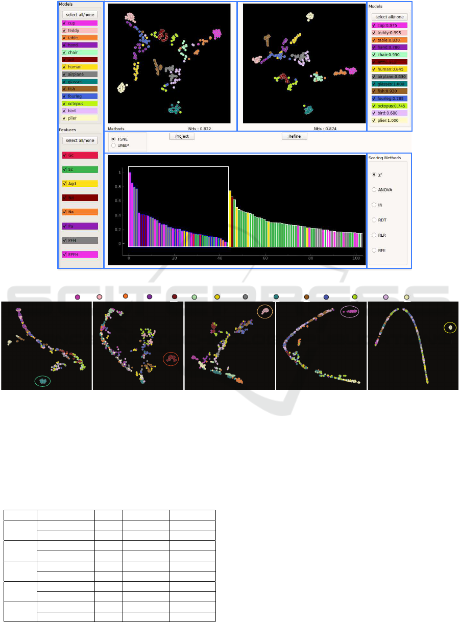
Figure 5: A user-driven projection engineering tool and its six views (Sec. 4.3).

a) glasses: (Sc:1,PFH:1) b) ant: (Pa:1,FPFH:1,FPH:1) c) teddy: (Nd:2,Gc:1) d) cup: (Agd:1,FPFH:1) e) pliers: (PFH:1)

glasses

ant

teddy

cup

pliers

cup teddy table hand ant chair human airplane glasses fish fourleg octopus bird plierscupClasses:

Figure 6: Finding minimal number of feature-bins able to separate ﬁve shape classes from the rest of the database. Notation

name:i indicates that i bins of feature name are used.

greedy algorithm for feature selection. (2) It is too

coarse-grained: All features of the same type, e.g.,

the 24 shape-context Sc features are either selected

all, or ignored, when constructing the projection. (3)

Table 2: Performance of the greedy algorithm.

Round Search method NH

Time (secs) t-SNE runs

Exhaustive 0.831 459.74 255

Greedy 0.831 103.49 56

Exhaustive 0.830 452.12 255

Greedy 0.830 84.98 48

Exhaustive 0.829 453.70 255

Greedy 0.820 70.24 40

Exhaustive 0.832 445.47 255

Greedy 0.832 111.71 64

Exhaustive 0.824 447.66 255

Greedy 0.824 97.39 55

It is too simplistic: There are cases when, for in-

stance, we want to optimize for separation of certain

classes more, based on problem-speciﬁc constraints.

Hence, user input in deciding which feature combi-

nation leads to the optimal projection is crucial.

We next address question Q2, rephrased as: How

can we pick ‘good’ feature-bins (from the total set of

1870 bins) that separate classes in the way we desire

in a speciﬁc context? For this, we propose an interac-

tive tool based on feature scoring (Fig. 5) which con-

tains several views (1–6) that allow the user to explore

the effect of features on separating classes of shapes

in the database, and also select subsets of features that

lead to a desired, better, class separation. We explain

these views via an overview-and-details-on-demand

workﬂow, as follows:

Visual Exploration of 3D Shape Databases Via Feature Selection

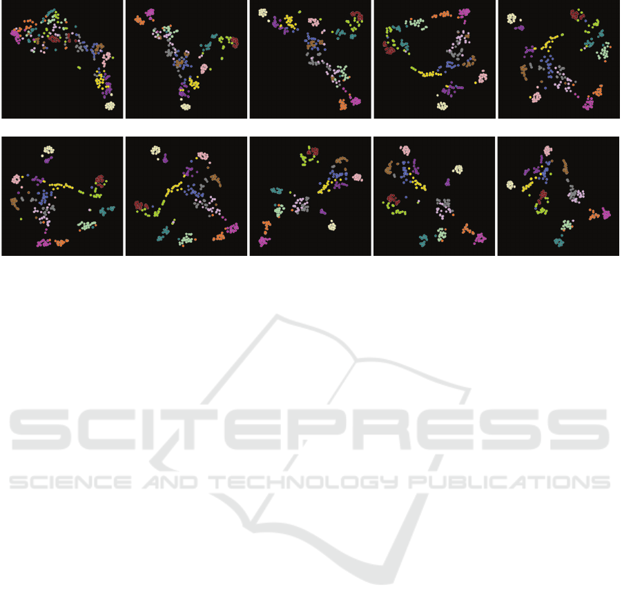
a) hand (10, 0, 0.584) b) table (5, 0, 0.745) c) airplane (3, 0, 0.750) d) octopus (11, 0, 0.816) e) fish (5, 0, 0.815)

f) glasses (5, 0, 0.825) g) bird (1, 0, 0.837) h) airplane, fish, bird

(

5, 0, 0.870)

i) airplane (

10, 0, 0.880)

j) all (

4, 8, 0.873)

Figure 7: Incremental creation of high-quality projection scatterplot that separates all classes well. In each step, a few feature-

bins (having high scores, count indicated in green) are selected to separate one or several classes from the rest, and a few

feature-bins (having low scores, count indicated in red) are removed from the selection. NH

at each step are rendered blue.

Model and Feature Selector (1): The user starts

by selecting the shape classes and feature types of

interest in this view. This allows them to specify

if they are interested in separating speciﬁc classes

(which are then to be selected) or, alternatively, inter-

ested in separating equally well all classes from each

other (in which case, all classes should be selected).

For instance, from our earlier experiments discussed

in Sec. 4.1, we saw that birds are hard to separate

from airplanes. The user can then select only these

two classes in view (1) to explore how to increase

their separation. Separately, one can select the feature

types (of the 8 computed ones) to use for creating the

scatterplot. This is useful to examine, or debug, the

effect of a speciﬁc feature type. Classes are categor-

ically color-coded, and the same colors are used in

the scatterplots (2, 5). Similarly, feature types are cat-

egorically color-coded with the same colors used in

the feature scoring view (3).

Original Scatterplot (2): This view shows a scatter-

plot using all shape classes vs all feature types chosen

in the selector (1). It acts as a starting point for the

exploration, which can next be reﬁned to e.g. pro-

duce better separation of desired classes or instances

(shapes) using the feature scoring views (3, 4) dis-

cussed next. Scatterplots can be computed either with

the t-SNE or UMAP (McInnes et al., 2018) projec-

tion methods. t-SNE spreads similar points better

over the available 2D space, but takes longer to com-

pute. UMAP creates denser clusters separated by

more whitespace, but is faster to execute. For a trade-

off of these two techniques, we refer to a recent sur-

vey (Espadoto et al., 2019).

Feature Scoring Views (3, 4): Each bar in the bar-

chart (3) shows the discriminative score of every el-

ement f

of the 1870-dimensional feature vector, i.e.,

how much f

contributes to separating class c

from

a few or from all other classes c

6= c

selected for

exploration in view (1), depending on the separation

control (6, discussed later). Colors identify to which

feature types the elements f

belong. For instance,

the several purple bars in Fig. 5(3) correspond to the

330 bins that the FPFH feature (colored purple in

Fig. 5(1)) has. Scores are computed with six scor-

ing methods(Rauber et al., 2015): chi-squared, one-

way ANOVA, Randomized Decision Trees (RDT),

Randomized Linear Regression (RLR), iterative re-

lief (IR), and Recursive Feature Elimination (RFE),

which can be chosen by the user in panel (4). The bar-

chart supports two tasks: First, it shows how the many

bins that each feature is represented by contributes to

the separation power of that feature. Secondly, it al-

lows ﬁne-grained examination of the effect of each

such bin on the class separation: Users can freely se-

lect speciﬁc bins (from the 1870 available ones) to

create a new projection. The selected bins are dis-

played with a blue border and listed, in decreasing

score order, before the unselected ones, in the bar-

chart. The new projection created by the user-selected

bins is shown in view (5).

Reﬁned Scatterplot (5): This scatterplot shows in-

stances from the classes selected in view (1), pro-

jected according to the speciﬁc feature-bins selected

in the barchart (3). This is thus a reﬁned view of

IVAPP 2020 - 11th International Conference on Information Visualization Theory and Applications

the original projection (1). By comparing the re-

ﬁned scatterplot with the original one, one can thus

see how ﬁne-grained selection of every single of the

1870 feature-vector components can improve the pro-

jection or parts thereof. In other words, obtaining

an optimal projection is achieved in two steps: First,

one can select entire features (in view 1). This corre-

sponds to considering or ignoring entire features that

capture different aspects of shape. Upon obtaining a

suitable projection, one can reﬁne it by selecting or

deselecting individual bins for the selected features.

This corresponds to considering or ignoring ranges

of the values of the features under exploration.

Separation Control (6): As mentioned, feature scor-

ing measures how well selected features separate a

class c

from one or several classes c

6= c

. The view

(6) allows controlling this. The view shows all shape

classes c

in the database. If all classes are selected

in view (6), scoring will measure how well a class c

is separated from each of the other classes c

6= c

. If

only one class c

is selected in (6), then scoring will

measure the separation of c

from ∪

j6=i

. This way,

one can ﬂexibly measure the separation of arbitrary

groups of classes rather than only the separation of

individual classes themselves.

4.4 Use-cases

We demonstrate the added value of our user-driven

projection engineering by answering several practical

questions, as follows.

A. What is the minimal number of feature values, and

which are these, that are sufﬁcient to separate a given

class of shapes from all others (Q3, Sec. 4.1)?

Figure 6 illustrates this use-case for the classes

glasses (a), ant (b), teddy (c), cup (d), and pliers

(e). For each class, we select the respective class in

the model selector (Fig. 5(1)) and use next the fea-

ture scoring view (Fig. 5(3)) and separation control

(Fig. 5(6)) to ﬁnd the feature values (bins of the 1870-

dimensional feature vector) that best separate this

class from the remaining ones. We assess separation

both visually, using the reﬁned projection (Fig. 5(5))

and its corresponding NH

score. We ﬁnd, this way,

that these classes can be separated very well from the

rest of the database by a maximally three, and some-

times just one, feature bin(s) of the 1870 computed

ones, as indicated in Fig. 6. This is, we believe, a

quite powerful (and novel) result as it indicates that

very little computational effort is needed for classify-

ing shapes in the Princeton Shape Database (and, by

extension, in other similar databases). In turn, this

can considerably increase the scalability of applica-

tions such as shape retrieval and classiﬁcation.

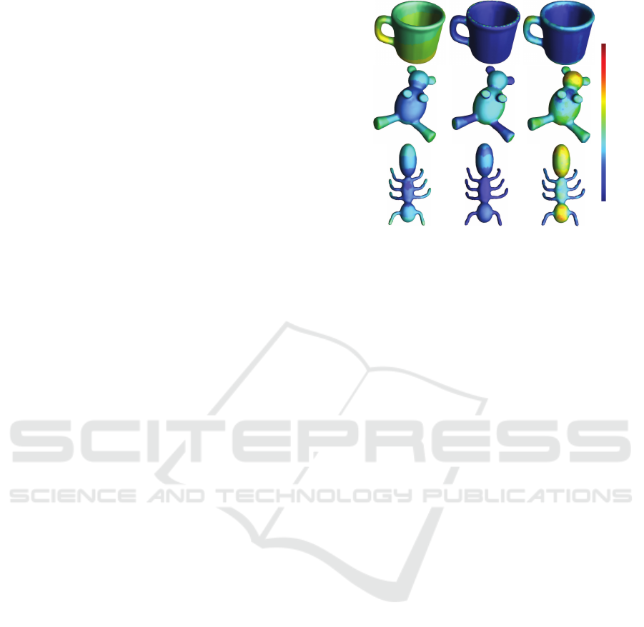
Agd Nd FPFH

cupteddyant

low

high

feature value

Figure 8: Feature-bins (Agd 6

bin, Nd 1

bin, and FPFH

bin) mapped on three shapes. This shows how these

speciﬁc feature bins can effectively separate these shapes.

B. How can we explain the discriminatory power of

the features found in use-case A?

The computed feature scoring and the clear separation

shown in the reﬁned projection scatterplots (Fig. 6)

are, in principle, enough to let us choose the mini-

mal set of feature-bins needed to separate a class from

all others. However, it is useful to double-check and

explain this discriminatory power, to ensure that the

features found this way indeed reﬂect meaningful dif-

ferent properties of the respective shape classes. For

this, we choose shapes from the analyzed classes in

use-case A and color them by the values of the fea-

tures found in the same step to be strongly character-

istic of speciﬁc classes. Figure 8 shows this for three

such shapes and feature-bins, respectively. As visi-

ble, the three feature-bins take indeed different values

for the three shapes. Atop of this insight (which we

already knew from the analysis shown in Fig. 6), we

also see now that the Nd feature has indeed low values

on thin shape parts and large values on thick ones, re-

spectively. Similarly, we see that the Agd is large for

shape protrusions (e.g. ant and teddy legs) but is small

for central shape parts (e.g. teddy rump). The FPFH

feature is harder to interpret visually; still, we can see

how it gets high values on roughly round shape parts

(teddy head and ant’s ﬁrst and last segments) and low

values elsewhere.

C. How can we create a good scatterplot which sepa-

rates well all classes?

Figure 7 shows an example workﬂow for this task.

We start here with a scatterplot that uses all 1870 fea-

tures. Next, we search, using the feature scoring view

(Fig. 5(3)), for the feature-bins that are most discrimi-

natory, i.e., have highest scores, for each of the classes

in our database, starting with the hand class (we could

start from any other class). As we progress investigat-

Visual Exploration of 3D Shape Databases Via Feature Selection

ing subsequent classes, we add feature-bins which are

discriminatory for these newly visited classes. At the

end, when we have considered all classes, we also re-

move features, from the already added ones, which

have low scores (that is, bring the least discrimina-

tion value or even work adversely for this task). The

entire process can be done in one to two minutes.

The different images in Fig. 7 show us how the qual-

ity (NH

value) of the scatterplot almost monotoni-

cally improves as we add more feature-bins by con-

sidering new classes. Note that, in this process, we

may visit a certain class several times (e.g. airplane),

as features that score high for it may appear several

times during the exploration as we add other classes.

The ﬁnal result (Fig. 7j) contains all 14 classes, has

a value NH

= 0.873, and is obtained with a total set

of 51 feature-bins. Note that this ﬁnal NH

value is

higher than the one we found by the exhaustive search

(NH

= 0.831, Tab. 1). Indeed, our manual search is

more ﬁne-grained, as it allows us to consider individ-

ual feature-bins (of the 1870 in total), whereas the au-

tomatic search only considered entire features (of the

8 in total). Also, note that obtaining this result by ex-

haustive search would be prohibitively expensive, as

this would involve searching all 2

1870

combinations.

5 DISCUSSION

We discuss next several aspects of our method, as fol-

lows:

Dimensionality Reduction: Currently, we directly

reduce dimensionality of our 1870-dimensional fea-

ture vector to 2D using either t-SNE or UMAP. How-

ever, this may be too hard a task for these projection

methods to perform, while in the same time preserv-

ing neighborhoods. Another approach is to use more

dedicated methods, such as autoencoders, to reduce

dimensionality to a lower value, and then project this

low-dimensional dataset to 2D using t-SNE or UMAP.

However, it has to be checked whether this approach

can yield ﬁnal 2D scatterplots that better preserve

the structure of the shape database. Concerning the

choice of projection techniques, we used t-SNE and

UMAP as these techniques are known for their abil-

ity to separate well, in the visual space, clusters of

similar observations, as opposed to other projection

techniques (Espadoto et al., 2019).

Scalability: Our method depends on two key param-

eters in this respect, namely the number of shapes in

the database to be explored, and the number of fea-

tures which are extracted from each shape. From

a computational viewpoint, feature extraction can be

done ofﬂine, as shapes are changed and/or new shapes

are added to the database. Since, typically, shape

databases do not change with a high frequency, such

an ofﬂine extraction can be done without impeding

the performance of the end user. Moreover, features

can be extracted in parallel, both among themselves

and over different shapes. We compute the t-SNE pro-

jection using the scikit-learn implementation, which

projects several hundreds of instances in a few sec-

onds; the UMAP implementation, provided by the au-

thors (McInnes et al., 2018), works in real time for

this dataset size. If needed, other, faster projections

can be used (Pezzotti et al., 2017). From a visualiza-

tion viewpoint, the scatterplot, barchart, and matrix

plot metaphors we use scale well to hundreds of thou-

sands of points (shapes) and tens of features.

Evaluation: One important aspect concerning our

proposal is evaluating its effectiveness for different

types of tasks and users. In detail, we identify end

users, for whom tasks involve getting an overview of a

shape database, ﬁnding similar groups of shapes, ﬁnd-

ing which features make two shape groups similar (or

different), and ﬁnding outlier shapes; and technical

users, for whom tasks involve selecting a small set of

features able to create effective visualizations for the

ﬁrst user group. We consider such evaluations to be

part of future work.

6 CONCLUSION

We have presented an interactive visual analytics sys-

tem for exploring 3D shape databases for CBSR ap-

plications. After reducing shapes to high-dimensional

feature vectors following standard feature extraction,

we visualize the similarity structure of a database by

using dimensionality reduction. To this end, we offer

several mechanisms for creating projections in which

different shape classes are separated well from each

other. First, we use a scagnostics approach to gener-

ate near-optimal projections based on maximizing the

quality of resulting projections, using a greedy heuris-

tic to optimize the search for suitable feature-sets.

Next, we propose a visual analytics approach to en-

able users to select a small feature subset for separat-

ing speciﬁc classes, generate high-separation projec-

tions for all classes, and gauge the separation power

(thus, added-value) of all available features. We show

that this visual analytics approach allows generating

projections with better separation quality than auto-

matic approaches, and also helps ﬁnding both dis-

criminating features (to be used in a CBSR system)

and confusing features (of little value for such sys-

tems). Our approach can be applied to any 3D shape

database and feature-set, allowing CBSR engineers to

IVAPP 2020 - 11th International Conference on Information Visualization Theory and Applications

streamline the process of designing and selecting ef-

fective features for shape classiﬁcation and retrieval.

We demonstrate our work on a real-world 3D shape

database.

Several extensions of this work are possible, as

follows. First and foremost, performing a user study

to gauge how well our approach can support explo-

ration tasks of typical end users, is an important addi-

tion. Secondly, since our approach is generic, it could

be used to optimize feature selection in other applica-

tions beyond CBSR, e.g., in image classiﬁcation.

REFERENCES

Aim@Shape (2019). Aim@shape digital shape workbench

5.0. http://visionair.ge.imati.cnr.it.

Belongie, S., Malik, J., and Puzicha, J. (2001). Shape con-

text: A new descriptor for shape matching and object

recognition. In Proc. NIPS, pages 831–837.

Bustos, B., Keim, D., Saupe, D., Schreck, T., and Vranic, D.

(2005). Feature-based similarity search in 3D object

databases. ACM Comput Surv, 37(4):345–387.

Cyr, C. M. and Kimia, B. B. (2001). 3D object recognition

using shape similiarity-based aspect graph. In Proc.

IEEE ICCV, pages 254–261.

Espadoto, M., Martins, R., Kerren, A., Hirata, N., and

Telea, A. (2019). Towards a quantitative survey

of dimension reduction techniques. IEEE TVCG.

doi:10.1109/TVCG.2019.2944182.

Feng, C., Jalba, A. C., and Telea, A. C. (2016). Improved

part-based segmentation of voxel shapes by skeleton

cut spaces. Mathematical Morphology –Theory and

Applications, 1(1).

ITI DB (2019). The informatics & telematics institute

database. http://3d-search.iti.gr/3DSearch/index.html.

Jalba, A., Kustra, J., and Telea, A. (2012). Surface and

curve skeletonization of large 3D models on the GPU.

IEEE TPAMI, 35(6):1495–1508.

Jalba, A., Kustra, J., and Telea, A. (2013). Computing sur-

face and curve skeletons from large meshes on the

GPU. IEEE TPAMI, 35(6):783–799.

Kalogerakis, E., Hertzmann, A., and Singh, K. (2010).

Learning 3D mesh segmentation and labeling. ACM

TOG, 29(4).

McInnes, L., Healy, J., and Melville, J. (2018). Umap: Uni-

form manifold approximation and projection for di-

mension reduction. arXiv:1802.03426.

NASA (2019). Nasa 3D resources. https://nasa3d.arc.nasa.

gov.

Paulovich, F. V., Nonato, L. G., Minghim, R., and Lev-

kowitz, H. (2008). Least square projection: A fast

high-precision multidimensional projection technique

and its application to document mapping. IEEE

TVCG, 14(3):564–575.

Peyre, G. and Cohen, L. (2005). Geodesic computations for

fast and accurate surface remeshing and parameteri-

zation. Progress in Nonlinear Differential Equations

and Their Applications, 63:151–171.

Pezzotti, N., Lelieveldt, B. P., van der Maaten, L., H

ollt,

T., Eisemann, E., and Vilanova, A. (2017). Approxi-

mated and user steerable t-SNE for progressive visual

analytics. IEEE TVCG, 23(7):1739–1752.

Rauber, P. E., da Silva, R. R. O., Feringa, S., Celebi, M. E.,

Falc

ao, A. X., and Telea, A. C. (2015). Interactive im-

age feature selection aided by dimensionality reduc-

tion. In Proc. EuroVA, pages 19–23.

Rusu, R. B., Blodow, N., and Beetz, M. (2009). Fast point

feature histograms (FPFH) for 3D registration. In

Proc. IEEE Intl. Conf. on Robotics and Automation,

pages 3212–3217.

ShapeNet (2019). ShapeNet online repository. https://www.

shapenet.org.

Shapira, L., Shamir, A., and Cohen-Or, D. (2008). Con-

sistent mesh partitioning and skeletonisation using

the shape diameter function. The Visual Computer,

24(4):249–262.

Shen, Y.-T., Chen, D.-Y., Tian, X.-P., and Ouhyoung, M.

(2003). 3D Model Search Engine Based on Lightﬁeld

Descriptors. In Eurographics 2003 - Posters. Euro-

graphics Association.

Shilane, P., Min, P., Kazhdan, M., and Funkhouser, T.

(2004). The Princeton shape benchmark. In Proc.

SMI, pages 167–178. http://shape.cs.princeton.edu/

benchmark.

Shneiderman, B. (1996). The eyes have it: A task by

data type taxonomy for information visualizations. In

Proc. IEEE Symp. on Visual Languages, pages 336–

343.

Shtrom, E., Leifman, G., and Tal, A. (2013). Saliency de-

tection in large point sets. In Proc. IEEE ICCV, pages

3591–3598.

Su, H., Maji, S., Kalogerakis, E., and Learned-Miller, E.

(2015). Multi-view convolutional neural networks for

3D shape recognition. In Proc. IEEE ICCV, pages

945–953.

Tangelder, J. and Veltkamp, R. (2008). A survey of content

based 3D shape retrieval methods. Multimedia Tools

and Applications, 39(3):441–471.

Tasse, F., Kosinka, J., and Dodgson, N. (2015). Cluster-

based point set saliency. In Proc. IEEE ICCV, pages

163–171.

Tukey, J. and Tukey, P. (1988). Computer graphics and ex-

ploratory data analysis: An introduction. In The Col-

lected Works of John W. Tukey: Graphics: 1965-1985.

TurboSquid, Inc. (2019). Turbosquid shape repository.

https://www.turbosquid.com.

van der Maaten, L. and Hinton, G. (2008). Visualizing high-

dimensional data using t-SNE. J Mach Learn Res,

(9):2579–2605.

Verma, V. and Snoeyink, J. (2009). Reducing the mem-

ory required to ﬁnd a geodesic shortest path on a large

mesh. In Proc. ACM GIS, pages 227–235.

Wattenberg, M. (2016). How to use t-SNE effectively. https:

//distill.pub/2016/misread-tsne.

Wilkinson, L., Anand, A., and Grossman, R. (2006). High-

dimensional visual analytics: Interactive exploration

guided by pairwise views of point distributions. IEEE

TVCG, 12(6):1363–1372.

Visual Exploration of 3D Shape Databases Via Feature Selection