FSSSD: Fixed Scale SSD for Vehicle Detection

Jiwon Jun

1 a

, Hyunjeong Pak

and Moongu Jeon

1 b

Gwangju Institute of Science and Technology, 123 Cheomdangwagi-ro, Buk-gu, Gwangju, South Korea

Korea Culture Technology Institute, 123 Cheomdangwagi-ro, Buk-gu, Gwangju, South Korea

Keywords:

Vehicle Detection, Object Detection, Surveillance System.

Abstract:

Since surveillance cameras are commonly installed in high places, the objects in the taken images are relatively

small. Detecting small objects is a hard issue for the one-stage detector, and its performance in the surveillance

system is not good. Two-stage detectors work better, but their speed is too slow to use in the real-time system.

To remedy the drawbacks, we propose an efﬁcient method, named as Fixed Scale SSD(FSSSD), which is an

extension of SSD. The proposed method has three key points: high-resolution inputs to detect small objects, a

lightweight Backbone to speed up, and prediction blocks to enrich features. FSSSD achieve 63.7% AP at 16.7

FPS in the UA-DETRAC test dataset. The performance is similar to two-stage detectors and faster than any

other one-stage method.

1 INTRODUCTION

As the architecture of deep convolutional neural net-

works(DCNN) has been evolved a lot recently, the

object detection algorithms using DCNN also have

been advanced signiﬁcantly. Object detection has

evolved into two streams depending on the applica-

tion. Two-stage detectors such as Faster-RCNN(Ren

et al., 2015), FPN(Lin et al., 2017), and Mask R-

CNN(He et al., 2017), are often used where the accu-

racy is more important. On the other hand, if real-time

processing is more important, efﬁcient one-stage de-

tectors such as SSD(Liu et al., 2016), YOLO(Redmon

et al., 2015) are commonly used.

Which of those two methods has been more fre-

quently used for vehicle detection? According to

the results of UA-DETRAC benchmark(Wen et al.,

2015), most of the high ranked detectors are based

on two-stage detectors. Why researchers commonly

have used two-stage detectors, not one-stage detec-

tors? Since the surveillance cameras are installed high

beside trafﬁc lights and signs, the sizes of the taken

images of objects are small. One-stage detectors do

not detect small objects well, so that the issue is fatal.

Two-stage detectors seem better than one-stage

detectors, but there exists a critical weak-point as the

execution speed is too slow for a real-time system.

https://orcid.org/0000-0002-9100-3471

https://orcid.org/0000-0002-2775-7789

All high ranked two-stage detectors in UA-DETRAC

benchmark runs at speeds between 0.1 frames per sec-

ond(FPS) and 10 FPS when detecting 960 × 540 im-

ages. It is not enough for real-time processing since

most surveillance videos are 24 FPS or higher.

To this end, we propose an efﬁcient one-stage de-

tector, named as ﬁxed scale SSD(FSSSD), for real-

time vehicle detection in surveillance videos. Our

main contribution can be summarized as follows:

- Use High-resolution Images as Input. One-stage

methods require a ﬁxed size input for correct ex-

ecution. For example, SSD resizes the inputs as

300 × 300 or 512 × 512. The resolution of surveil-

lance cameras is usually bigger than the ﬁxed sizes.

Therefore resizing the image smaller is included in

preprocessing. It makes small objects smaller, which

makes one-stage methods even weaker. In this work,

we do not resize the images and use the original size

to avoid the issue.

- Design a Light Architecture for Real-time Detec-

tion. Using large size inputs improves performance

on detecting small objects, but it makes the execu-

tion speed signiﬁcantly slower. To make feasible real-

time detection, we design a lightweight architecture

using ShufﬂeNetV2(Ma et al., 2018) and prediction

blocks(Lee et al., 2017).

- Use Fixed Scales for Freely Changing the Input

Size. Choosing the scales is very important to one-

stage methods for correct detection. Traditional one-

stage detectors using the SSD framework use relative

336

Jun, J., Pak, H. and Jeon, M.

FSSSD: Fixed Scale SSD for Vehicle Detection.

DOI: 10.5220/0008950503360342

In Proceedings of the 15th International Joint Conference on Computer Vision, Imaging and Computer Graphics Theory and Applications (VISIGRAPP 2020) - Volume 5: VISAPP, pages

336-342

ISBN: 978-989-758-402-2; ISSN: 2184-4321

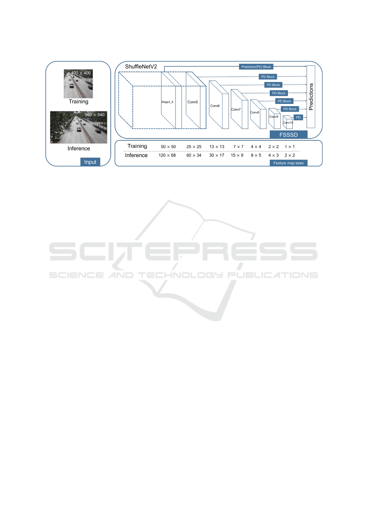
Figure 1: The architecture of FSSSD: since ﬁxed scale detection can change the input size, training time can be signiﬁcantly

reduced by using training patches which is smaller than images used for the inference time.

scales which help detect all size of objects in an im-

age. Since the scales is relative, the scale informa-

tion of each feature map depends on the input size

as shown in Table 1. Therefore, the detectors are not

able to detect properly if the input size is changed.

However, if the input size can be changed, there are

lots of advantages such as decreasing training time

by using small size inputs or execution time by using

cropped images. So we use ﬁxed scales instead of rel-

ative scales to take the advantages. This is described

in more detail in Sec. 3.1.4.

2 RELATED WORKS

2.1 Two-stage Detection

Two-stage detectors use region proposals, such as

selective search(Uijlings et al., 2013) or RPN(Ren

et al., 2015), to obtain proposals and detect each pro-

posal with deep neural networks. R-CNN(Girshick

et al., 2014) is the ﬁrst two-stage detection model,

and its accuracy is signiﬁcantly better than traditional

methods. Across Fast R-CNN(Girshick, 2015) and

Faster R-CNN, two-stage methods have developed

greatly, and models such as FPN and Mask R-CNN

are continuously proposed for more accurate detec-

tion. However, two-stage method has a fatal disad-

vantage: slow computation. Faster R-CNN operates

at only 7 FPS with high-end hardware.

2.2 One-stage Detection

One-stage detection is introduced to solve the slow

speed of two-stage detectors. The most famous one-

stage detectors are SSD and YOLO. Between them,

SSD is more widely used due to the convenience of

structure use. The detectors using the SSD frame-

work predict category scores and box offsets for mul-

tiple objects based on feature maps. By completely

eliminating the proposal generating process and en-

capsulating it with classiﬁcation stage, the detectors

have achieved similar accuracy to two-stage detectors

at feasible speed. But they are not good at detect-

ing small objects because feature maps for detecting

small objects do not have enough features.

3 METHODS

This section explains proposed FSSSD for vehicle

detection in the surveillance system and its train-

ing strategy. After that, we describe dataset-speciﬁc

model details.

3.1 Fixed Scales SSD (FSSSD)

The proposed FSSSD is based on SSD frame-

work(Liu et al., 2016). we accept the concepts; multi-

scale feature maps, default boxes, convolutional pre-

dictors, and scales. The main modiﬁcations are a

high-resolution input, a lightweight backbone for fast

processing, prediction blocks(Lee et al., 2017) to en-

rich the features, and ﬁxed scales for fast training.

3.1.1 Use High-resolution Images for Small

Object Detection

Most one-stage methods use the small input size, i.e.,

300 × 300 or 512 × 512. Because the resolution of

surveillance videos is larger than resized resolution,

resizing the image is required before the detecting

FSSSD: Fixed Scale SSD for Vehicle Detection

337

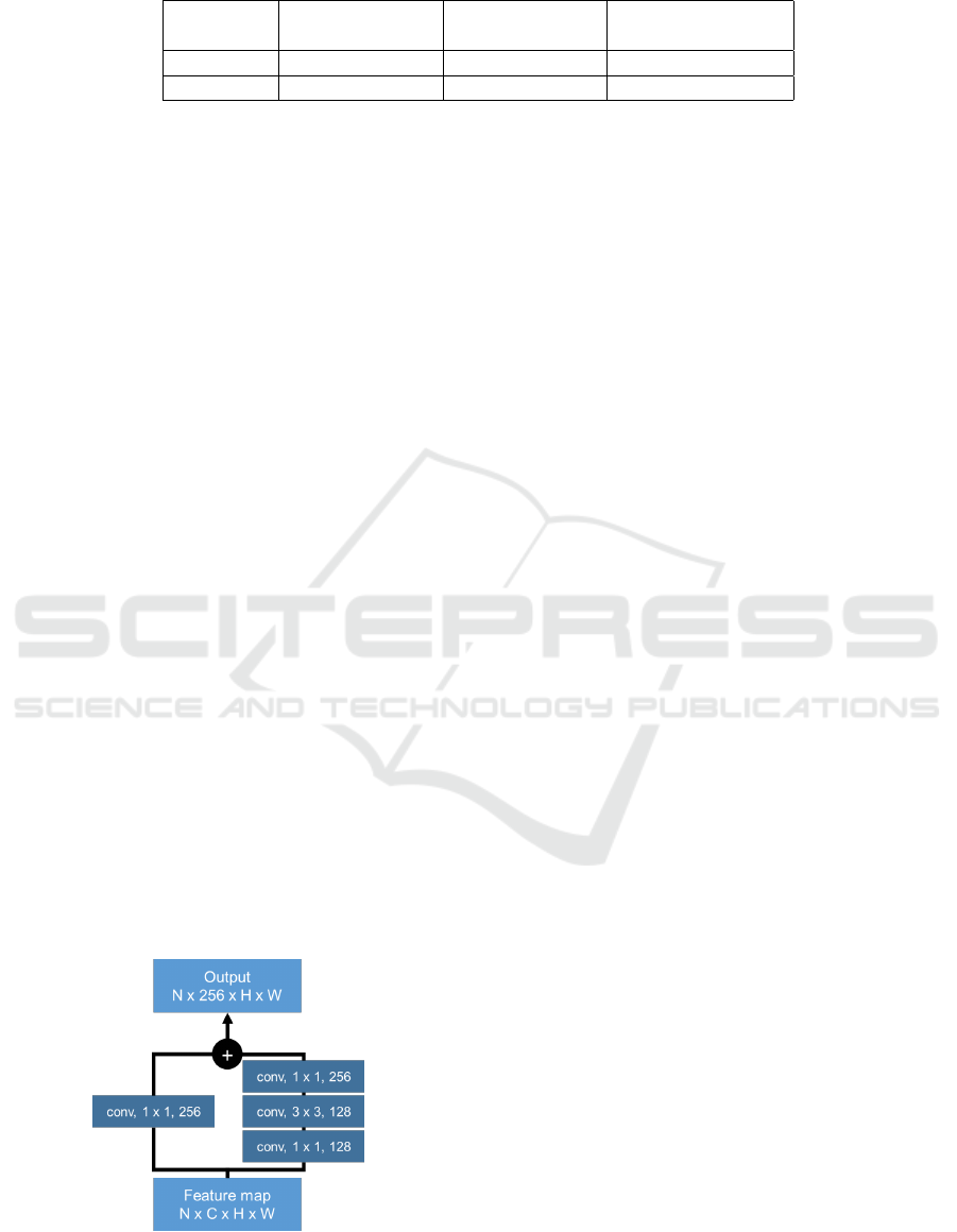
Table 1: Comparison between relative and ﬁxed scales.

Input size

1st source

1st scale in SSD 1st scale in FSSSD

feature map size

400 × 400 50 × 50 (f ) 40 × 40 (0.1) 40 × 40

960 × 540 120 × 68 (f

) 96 × 54 (0.1) 40 × 40

process. It aggravates the performance of the one-

stage detectors on small objects. To solve the issue,

we use high-resolution images as input.

3.1.2 Lightweight Backbone

Although high-resolution inputs improve perfor-

mance on detecting small objects, it makes the de-

tector slows down signiﬁcantly as the number of pre-

dictions increases in proportion to the input size.

To solve this, we use a lightweight network for the

backbone network to reduce the number of computa-

tions and not to lose performance. We employ Shuf-

ﬂeNetV2 for the backbone of FSSSD since it is faster

and more accurate than other lightweight networks.

Among the variances, we apply ShufﬂeNetV2 1x in

consideration of speed and accuracy tradeoff.

3.1.3 Prediction Blocks

Another reason for low performance of small ob-

ject detection is that the feature map do not contain

enough features for detecting objects. To overcome

the weakness, we apply the prediction blocks(Lee

et al., 2017) before passing predicting convolution ﬁl-

ters as Figure 1. Prediction blocks enrich features in

feature maps and provide larger receptive ﬁelds. With

large receptive ﬁelds, the feature maps contain more

contextual information. As shown in Hu et al.(Hu

and Ramanan, 2017), contextual information is very

helpful for detecting small objects. For this reason,

FSSSD can achieve better results than other one-stage

detectors. The structure of prediction Block is shown

in Figure 2.

Figure 2: Prediction Block.

3.1.4 Fixed Scales for Reducing Training Time

It is trivial that training takes a long time because of

the big size of the input. In order to reduce long train-

ing time, we use small size of cropped patches in-

stead of original size of input for training. To make

this work properly, we use ﬁxed scales instead of rel-

ative scales. The scales are very important in SSD

framework because the scale information which is

contained in the feature maps depends on the scales.

Since SSD uses relative scales, the scale values are

changed when the input size is changed, as shown

in Table 1. If a 960 × 540 resolution image passes

SSD model which is trained with 400×400 resolution

samples, the predictions are inaccurate because of the

scale difference between f and f

. However, FSSSD

can perform correct predictions because of the ﬁxed

scale, even if the input size is changed.

Using ﬁxed scales has a risk: the objects which

are bigger than the largest scale can not be detected.

Therefore, ﬁxed scales and the size of the patches

should be determined by considering the scale of the

objects. In the surveillance system, most vehicles are

small since the cameras are located in high places

such as over the trafﬁc lights or signs. So we assumed

that every object is smaller than half the size of the

image. According to the assumption, we set the size

of patches as 400 × 400 for input size of 960 × 540

and the ﬁxed scales adapted to the patch size.

3.1.5 Auxiliary Network for Changing Input

Size Freely

The auxiliary network in SSD is designed using the

ﬁxed input size. Especially, the feature maps close

to head are resized by using convolution ﬁlters with-

out strides. This way do not work as intended when

the input size is changed. For example, the 3 × 3 fea-

ture map becomes 1 ×1 feature map through the 3×3

convolution ﬁlters without padding. The width and

height of the feature map are reduced by one-third.

However, the 5 × 5 feature map becomes 3 × 3 fea-

ture map through the same convolution ﬁlters. The

size is not intended, so the prediction results would

be inaccurate. As we need to change the input size,

we design the auxiliary network taking these issues

into account. If it is necessary to reduce the size of a

feature map, we only use strides of convolution ﬁlters.

VISAPP 2020 - 15th International Conference on Computer Vision Theory and Applications

338

3.2 Training

Since FSSSD is based on SSD, most of the features

such as matching strategy, training objects, etc. are

the same.

3.2.1 Dataset

We use UA-DETRAC(Wen et al., 2015) taken by

surveillance cameras for 10 hours with the 960 × 540

resolution. Since the dataset consists of the images

of 24 different locations and contains 1.21 million

labeled bounding boxes with four vehicle types(car,

van, bus, and other), it is an optimized dataset for

experimenting with vehicle detection. According to

Wen et al. (Wen et al., 2015), most objects in the

dataset are smaller than 300 ×300. Therefore, the size

of patches, 400×400, is appropriate to cover all kinds

of scales.

The evaluation of UA-DETRAC uses the

IOU=0.7

metric. A feature of the evaluation is that

the predicting the type of vehicles is not included in

the metric. Although the type of vehicles does not

affect the evaluation score, increasing the number of

categories helps improve the performance. So FSSSD

uses the type information for accurate detection.

There are 60 sequences for training, and 40 se-

quences for testing. Because there is no dataset

for validation, 10 sequences were randomly selected

from the training set and used as a validation set.

3.2.2 Data Augmentations

Each training patch is randomly sampled by following

Algorithm 1. After the sampling step, each sampled

patch is horizontally ﬂipped with a probability of 0.5

after some photo-metric distortions.

3.2.3 Multi-scale Feature Maps and Scales

Multi-scale feature maps are the most important fea-

ture in the SSD framework for detecting objects of

various sizes. The feature maps close to the bottom

are used to detect small objects, whereas the feature

maps close to the head are used to detect big objects.

Considering the input size, 400 × 400, we selected 7

multi-scale feature maps, two of them from the back-

bone and the others from the auxiliary network. For

each feature map f

is a pair with a ﬁxed scale s

Similar to SSD, the smallest scale s

is set as 40, the

0.1 of the input size, and the largest scale s

is set

as 360, the 0.9 of the input size. The scales of other

feature maps are computed as:

= s

− s

m − 1

(k − 1), k ∈ [1, m] (1)

Algorithm 1: Data Augmenting: Get a patch of a speciﬁc

size.

Input I (images tensor), L (labels tensor), size (in-

put size)

Output I

, L

n ← 1

FLAG ← 0

while FLAG = 0 do

rand ← randomly select among 0.1, 0.3, 0.5, 0.7,

0.9

tmp

, L

tmp

← RandomCrop(I, L, size)

if Overlap(L, L

tmp

) > rand then

, L

← I

tmp

, L

tmp

FLAG ← 1

else

if n > 50 then

, L

← Resize(I, L, size)

FLAG ← 1

end if

n ← n + 1

end while

m is the number of multi-scale feature maps and m = 7

for FSSSD.

3.2.4 Default Boxes

Each convolution predictor predicts the conﬁdences

of all categories (classiﬁcation) and the locations by

x, y, width, height (localization). Default boxes have

several default shapes to help with the localization.

Each feature maps have different default box shapes,

also called as aspect ratios. The 1st, 6th, and 7th fea-

ture maps have 3 aspect ratios; {1,2,

} and the other

feature maps have 5 aspect ratios; {1, 2, 3,

4 EXPERIMENTS

We used PyTorch (Paszke et al., 2017) for imple-

menting the networks. The backbone network, Shuf-

ﬂeNetV2, was pre-trained on the ILSVRC CLS-LOC

dataset(Russakovsky et al., 2015). We add batch nor-

malization layers to all convolution layers in the aux-

iliary network because batch normalization helps sta-

ble optimization, as pointed out in (Santurkar et al.,

2018). We ﬁne-tuned FSSSD using SGD optimizer

with batch size 32, initial learning rate 1e-3, momen-

tum 0.9, and weight decay 5e-4. The learning rate

was reduced by one-tenth twice, 150,000 iterations

and 180,000 iterations. We trained on a 1080ti GPU,

Intel(R) Xeon(R) CPU E5-2620 v4 @ 2.10GHz.

FSSSD: Fixed Scale SSD for Vehicle Detection

339

Table 2: UA-DETRAC test benchmark results.

Method

AP(%)

FPS

full easy medium hard cloudy night rainy sunny

Two-stage methods

(Girshick et al., 2014) 49.0 59.3 54.1 39.5 59.7 39.3 39.1 67.5 0.1

(Ren et al., 2015) 58.5 82.8 63.1 44.3 66.3 69.9 45.2 62.3 11.1

(Wang et al., 2017) 68.0 89.7 73.1 53.6 72.4 73.9 53.4 83.7 9.1

(Dai et al., 2016) 69.9 93.3 75.7 54.3 74.4 75.1 56.2 84.1 6

One-stage methods

(Redmon and Farhadi, 2017) 57.7 83.3 62.3 42.4 58.0 64.5 47.8 69.8 -

FSSSD 63.7 83.5 68.2 51.0 72.6 62.0 50.5 77.5 16.7

FSSSD-fast 60.5 80.4 65.5 47.4 67.9 59.5 47.9 76.0 31.7

Finally, we achieved 63.7% AP at 16.7 FPS on the

UA-DETRAC benchmark. Table 2 summarizes the

comparison with the baseline results. The result of

FSSSD is better than all one-stage detectors, such as

YOLO2(Redmon and Farhadi, 2017), and even Faster

R-CNN. Although R-FCN(Dai et al., 2016) shows

better accuracy, the speed of FSSSD is 2.8 times faster

than R-FCN.

4.1 Necessary of Prediction Blocks

First, we studied the effect of the prediction blocks.

And we also studied whether the batch normalization

is important or not. When batch normalization was

not applied, the model did not converge. We also

tested with a smaller learning rate, 1e-4, the model

still diverge so we could not measure the results. So

we concluded that the batch normalization is essen-

tial to train models. We also tested the model without

the prediction blocks. The accuracy rate was 55.3%,

which is 7.6% lower than FSSSD. It is clearly shown

in Figure 4.

Table 3: Effects of Batchnorm and Prediction Blocks.

FSSSD

Use Batchnorm X X

Prediction Blocks X

UA-DETRAC AP NaN 55.3% 63.7%

This huge difference is due to the lightweight

backbone. VGG16(Simonyan and Zisserman, 2014),

the backbone of SSD, has 5% higher top-1 accu-

racy than ShufﬂeNetV2 1x in ILSVRC. Therefore

we know the feature maps from ShufﬂeNetV2 do

not have enough features to classify images. Al-

though there are not sufﬁcient features in the feature

maps, FSSSD showed good result with the prediction

blocks, which is shown in this study.

4.2 Training Speed

We used ﬁxed scales to train the model faster. To de-

termine the degree of acceleration, we measured the

average time taken for training. When we experi-

mented with the same environment except for the in-

put size, the speed of training using the small patches

was 0.2748 sec/batch and the speed of training with

the original size patches was 0.4460 sec/batch. The

training speed using the small patches is about 1.63

times faster, which makes the difference in total train-

ing time about 9.51h.

4.3 How to Speed up FSSSD?

The speed of FSSSD shows 16.7 FPS, which is not

enough to be called real-time. But there are various

ways to speed up the model.

4.3.1 Reduce the Number of Categories

The ﬁrst way to speed up FSSSD is by using only

one category. We used category information as men-

tioned above Sec. 3.2.1. There are 49054 predictions

for a class with 960 × 540 resolution of the input.

Merging categories, that is, eliminating the three cate-

gories, has the advantage of speed as it reduces about

150k predictions. We call the model with one cate-

gory as FSSSD-fast. It showed a little low accuracy

than FSSSD, but the processing speed has doubled.

FSSSD-fast is a meaningful model since the model is

the fastest detector in UA-DETRAC benchmarks.

4.3.2 Discard Unnecessary Region

As with the training stage, FSSSD is capable of freely

changing the size of the input. Therefore, if we know

the unnecessary area of the image, removing the re-

gion is possible. Since changing the input size does

not change any parameters of the model, the detection

performance remains the same as shown in Figure 3.

VISAPP 2020 - 15th International Conference on Computer Vision Theory and Applications

340

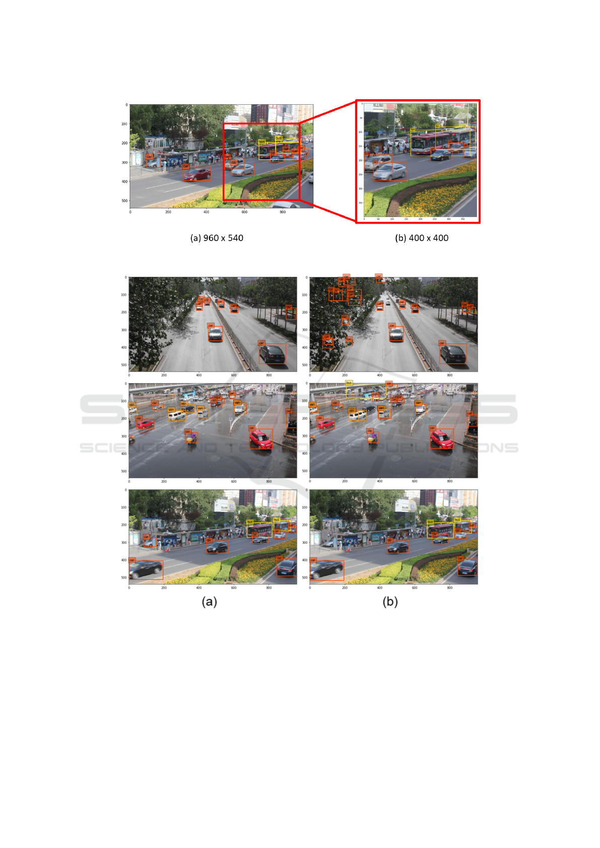
Figure 3: Detection results of FSSSD with input size (a) 960 × 540 and (b) 400 × 400.

Figure 4: Detection examples on the UA-DETRAC test dataset: (a) with prediction blocks and (b) without prediction blocks.

With 400 × 400 resolution of the input, the speed of

FSSSD is 32.1 FPS, which is enough to use in real-

time vehicle detection.

5 CONCLUSIONS

In this paper, we propose an efﬁcient one-stage detec-

tor, named as FSSSD, for real-time vehicle detection

in the surveillance system. We use high-resolution

images to detect small vehicles, the lightweight back-

FSSSD: Fixed Scale SSD for Vehicle Detection

341

bone to reduce execution time and the prediction

blocks to enrich the source feature maps. By com-

bining them, FSSSD runs at 16.7 FPS, which is faster

than any two-stage detectors and achieves 63.7% AP,

which is the highest one among all one-stage detec-

tors.

ACKNOWLEDGEMENTS

This work was partly supported by Institute of Infor-

mation & Communications Technology Planning &

Evaluation(IITP) grant funded by the Korea govern-

ment(MSIT) (No.2014-3-00077, AI National Strat-

egy Project) and the National Research Foundation

of Korea (NRF) grant funded by the Korea govern-

ment(MSIT) (No. 2019R1A2C2087489).

REFERENCES

Dai, J., Li, Y., He, K., and Sun, J. (2016). R-FCN: object de-

tection via region-based fully convolutional networks.

CoRR, abs/1605.06409.

Girshick, R. (2015). Fast r-cnn. In Proceedings of the 2015

IEEE International Conference on Computer Vision

(ICCV), ICCV ’15, pages 1440–1448, Washington,

DC, USA. IEEE Computer Society.

Girshick, R., Donahue, J., Darrell, T., and Malik, J. (2014).

Rich feature hierarchies for accurate object detection

and semantic segmentation. In Proceedings of the

2014 IEEE Conference on Computer Vision and Pat-

tern Recognition, CVPR ’14, pages 580–587, Wash-

ington, DC, USA. IEEE Computer Society.

He, K., Gkioxari, G., Doll

ar, P., and Girshick, R. (2017).

Mask r-cnn. In Proceedings of the IEEE international

conference on computer vision, pages 2961–2969.

Hu, P. and Ramanan, D. (2017). Finding tiny faces. In Pro-

ceedings of the IEEE conference on computer vision

and pattern recognition, pages 951–959.

Lee, K., Choi, J., Jeong, J., and Kwak, N. (2017). Resid-

ual features and uniﬁed prediction network for single

stage detection. CoRR, abs/1707.05031.

Lin, T.-Y., Doll

ar, P., Girshick, R., He, K., Hariharan, B.,

and Belongie, S. (2017). Feature pyramid networks

for object detection. In Proceedings of the IEEE con-

ference on computer vision and pattern recognition,

pages 2117–2125.

Liu, W., Anguelov, D., Erhan, D., Szegedy, C., Reed, S.,

Fu, C.-Y., and Berg, A. C. (2016). Ssd: Single shot

multibox detector. In European conference on com-

puter vision, pages 21–37. Springer.

Ma, N., Zhang, X., Zheng, H.-T., and Sun, J. (2018). Shuf-

ﬂenet v2: Practical guidelines for efﬁcient cnn archi-

tecture design. In Proceedings of the European Con-

ference on Computer Vision (ECCV), pages 116–131.

Paszke, A., Gross, S., Chintala, S., Chanan, G., Yang, E.,

DeVito, Z., Lin, Z., Desmaison, A., Antiga, L., and

Lerer, A. (2017). Automatic differentiation in Py-

Torch. In NIPS Autodiff Workshop.

Redmon, J., Divvala, S. K., Girshick, R. B., and Farhadi, A.

(2015). You only look once: Uniﬁed, real-time object

detection. CoRR, abs/1506.02640.

Redmon, J. and Farhadi, A. (2017). Yolo9000: better, faster,

stronger. In Proceedings of the IEEE conference on

computer vision and pattern recognition, pages 7263–

7271.

Ren, S., He, K., Girshick, R., and Sun, J. (2015). Faster

r-cnn: Towards real-time object detection with region

proposal networks. In Cortes, C., Lawrence, N. D.,

Lee, D. D., Sugiyama, M., and Garnett, R., editors,

Advances in Neural Information Processing Systems

28, pages 91–99. Curran Associates, Inc.

Russakovsky, O., Deng, J., Su, H., Krause, J., Satheesh,

S., Ma, S., Huang, Z., Karpathy, A., Khosla, A.,

Bernstein, M., Berg, A. C., and Fei-Fei, L. (2015).

ImageNet Large Scale Visual Recognition Challenge.

International Journal of Computer Vision (IJCV),

115(3):211–252.

Santurkar, S., Tsipras, D., Ilyas, A., and Madry, A. (2018).

How does batch normalization help optimization?(no,

it is not about internal covariate shift). arXiv preprint

arXiv:1805.11604.

Simonyan, K. and Zisserman, A. (2014). Very deep con-

volutional networks for large-scale image recognition.

arXiv preprint arXiv:1409.1556.

Uijlings, J., van de Sande, K., Gevers, T., and Smeulders,

A. (2013). Selective search for object recognition. In-

ternational Journal of Computer Vision.

Wang, L., Lu, Y., Wang, H., Zheng, Y., Ye, H., and Xue,

X. (2017). Evolving boxes for fast vehicle detection.

CoRR, abs/1702.00254.

Wen, L., Du, D., Cai, Z., Lei, Z., Chang, M., Qi, H., Lim,

J., Yang, M., and Lyu, S. (2015). UA-DETRAC: A

new benchmark and protocol for multi-object detec-

tion and tracking. arXiv CoRR, abs/1511.04136.

VISAPP 2020 - 15th International Conference on Computer Vision Theory and Applications

342