
Deep Learning of Heuristics for Domain-independent Planning
Otakar Trunda
a
and Roman Bart
´
ak
b
Charles University, Faculty of Mathematics and Physics, Czech Republic
Keywords:
Heuristic Learning, Automated Planning, Machine Learning, State Space Search, Knowledge Extraction,
Zero-learning, STRIPS, Neural Networks, Loss Functions, Feature Extraction.
Abstract:
Automated planning deals with the problem of finding a sequence of actions leading from a given state to a
desired state. The state-of-the-art automated planning techniques exploit informed forward search guided by a
heuristic, where the heuristic (under)estimates a distance from a state to a goal state. In this paper, we present
a technique to automatically construct an efficient heuristic for a given domain. The proposed approach is
based on training a deep neural network using a set of solved planning problems from the domain. We use a
novel way of generating features for states which doesn’t depend on usage of existing heuristics. The trained
network can be used as a heuristic on any problem from the domain of interest without any limitation on
the problem size. Our experiments show that the technique is competitive with popular domain-independent
heuristic.
1 INTRODUCTION
Heuristic learning is a relatively new field which stud-
ies how machine learning (ML) can be used to con-
struct a heuristic used in informed forward-search al-
gorithms such as A* and IDA*. The objective is to
train a regression-based ML model to be able to es-
timate goal-distances of states and then to use the
trained model as a heuristic function during search.
Automated planning, which deals with finding
a sequence of actions leading to a goal state, ex-
ploits heuristics heavily. Domain-specific heuristics
are hand-tailored for a specific domain and hence they
are very efficient. However, developing them requires
tremendous human effort and access to expert knowl-
edge. Domain-independent heuristics are more pop-
ular in automated planners as they are designed once
and then they work across all domains. Nevertheless,
none of them works well on all domains. Again, a
significant human effort would be required to select
the best performing heuristic for the problem at hand,
otherwise the search might be inefficient. This issue
can partially be solved by using a portfolio-planner.
In this paper, we present a ML technique that au-
tomatizes the process of developing domain-specific
heuristics for planning. We work with the standard
STRIPS planing and we use supervised learning, with
a
https://orcid.org/0000-0002-7868-7039
b
https://orcid.org/0000-0002-6717-8175
a multi-layered feed-forward neural network as the
ML model. Expert knowledge about the domain is
extracted automatically from a set of training sam-
ples. Using ML techniques for this task can be advan-
tageous because in this particular case, the training
samples can be obtained without human assistance,
unlike in typical applications of ML where samples
need to be human-labeled.
Our technique falls into category of zero-learning
as the heuristic is constructed from scratch, without
any human-knowledge initially added. This approach
allows us to combine wide usability of domain-
independent heuristics with accuracy of domain-
specific ones without any assistance of a human ex-
pert.
Our main contribution is twofold. We propose a
novel way of assigning features to states based on
counting subgraphs of a graph-based representation
of the state. The method produces fixed-size fea-
ture vectors without depending on existing heuristics.
Second, we study the effect of the choice of loss func-
tion used during the training, on performance of the
learned heuristic during the search. We show that
Mean Squared Error (MSE) alone might not be the
best loss function for heuristic learning task, and also
that low error on training and test sets doesn’t au-
tomatically imply good performance of the learned
heuristic.
Trunda, O. and Barták, R.
Deep Learning of Heuristics for Domain-independent Planning.
DOI: 10.5220/0008950400790088
In Proceedings of the 12th International Conference on Agents and Artificial Intelligence (ICAART 2020) - Volume 2, pages 79-88
ISBN: 978-989-758-395-7; ISSN: 2184-433X
Copyright
c
2022 by SCITEPRESS – Science and Technology Publications, Lda. All rights reserved
79

2 BACKGROUND AND RELATED
WORKS
2.1 STRIPS Planning
We work with classical planning problems, that is,
with finding a sequence of actions transferring the
world from a given initial state to a state satisfying
certain goal condition (Nau et al., 2004). World states
are represented as sets of predicates that are true in
the state (all other predicates are false in the state).
For example the predicate at(r1, l1) represents infor-
mation that some object r1 is at location l1. Actions
describe how the world state can be changed. Each
action a is defined by a set of predicates prec(a) as
its precondition and two disjoint sets of predicates
eff
+
(a) and eff
−
(a) as its positive and negative ef-
fects. Action a is applicable to state s if prec(a) ⊆ s
holds. If action a is applicable to state s then a new
state γ(a, s) defines the state after application of a as
γ(a, s) = (s ∪ eff
+
(a)) − eff
−
(a) Otherwise, the state
γ(a, s) is undefined. The goal g is defined as a set of
predicates that must be true in the goal state. Hence
the state s is a goal state if and only if g ⊆ s.
The satisficing planning task is formulated as fol-
lows: given a description of the initial state s
0
, a set
A of available actions, and a goal condition g, is there
a sequence of actions (a
1
, . . . , a
n
), called a solution
plan, such that a
i
∈ A, a
1
is applicable to state s
0
, each
a
i
s.t. i > 1 is applicable to state γ(a
i−1
, . . . γ(a
1
, s
0
)),
and g ⊆ γ(a
n
, γ(a
n−1
, . . . γ(a
1
, s
0
)))? Assume that each
action a has some cost c(a). An optimal planning task
is about finding a solution plan such that the sum of
costs of actions in the plan is minimized.
In practice, the planning problem is specified in
two components: a planning domain file and a plan-
ning problem file. The domain file specifies the names
of predicates describing properties of world states and
actions that can be used to change world states. The
problem file then specifies a particular goal condition
and an initial state and hence it also gives the names
of used objects (constants) and their types.
In the rest of the text we use the following nota-
tion. P denotes a planning problem, s
P
0
denotes the
initial state of P, S
P
the set of all states of P, Dom(P)
a set of all planning problems from the same domain
as P and S
Dom(P)
a set of states of all problems from
the same domain as P. For a state s
P
∈ S
P
, h
∗
(s
P
) de-
notes the goal-distance of s
P
in P, i.e. the cost of the
optimal plan from s
P
, or ∞ if there is no path from s
P
to a goal state.
2.2 Heuristic Learning
A heuristic learning (HL) system works with a set
of training samples, where each training sample is a
pair (s
i
, h
∗
(s
i
)), s
i
is a state of some planning problem
and h
∗
(s
i
) is its goal-distance. The system involves a
ML model M that is trained to predict h
∗
(s
i
) from s
i
.
Most of ML models work with fixed-size real valued
vectors as their inputs, hence another component is
required that transforms states into this form. We call
this component a features generator and denote it by
F. We call F(s) the features of s, and h
∗
(s) the target
of s. There are several variants of HL based on their
usage scenarios:
Type I: several problems P
1
, P
2
, . . . P
j
and P from
the same domain are given as input and the task is
solving the problem P as quickly as possible. Time
required for generating the training data and training
the model is considered a part of the solving process.
The ML model is trained specifically for P, it is not
intended to work on different problems.
Type II: several problems P
1
, P
2
, . . . P
j
from the
same domain Dom are given and the task is solving
new problems from Dom. Time required for generat-
ing the training data and training the model is NOT
considered a part of the solving process. It is con-
sidered a pre-processing, or a domain analysis phase.
The ML model captures knowledge about the whole
domain, i.e., it can generalize to other, previously un-
seen problems from the same domain. The training
phase can in this case take several hours or even days.
After the model is trained, new problems from the
same domain can be solved quickly. The Type II HL
system requires a much more flexible features genera-
tor, as features of states of different problems must be
comparable. Those different problems might contain
different numbers of objects and might have different
goal conditions.
Type III: Training samples from several differ-
ent domains are given and the ML model serves as
a multi-domain heuristic, or a domain-independent
heuristic. To our best knowledge, no serious attempt
has been made in this area.
In this paper, we work with the Type II HL and our
approach is domain-independent in a sense that the
domain from which the training problems come might
be arbitrary. We conducted experiments on domains
without action costs but the technique is applicable to
domains with costs as well.
ICAART 2020 - 12th International Conference on Agents and Artificial Intelligence
80

2.3 Related Works
Many attempts have been made to utilize ML in plan-
ning or in general search (Jim
´
enez et al., 2012). ML
has been used to learn reactive policies (Groshev
et al., 2017; Mart
´
ın and Geffner, 2004; Groshev et al.,
2018), control knowledge (Yoon et al., 2008), for
plan recognition (Bisson et al., 2015) and for other
planning-related tasks (Konidaris et al., 2018). ML
tools are also often used to combine several heuris-
tics (Samadi et al., 2008; Fink, 2007) and in par-
ticular to help portfolio-based planners to efficiently
combine multiple search algorithms (Cenamor et al.,
2013). A lot of papers exist that utilize ML in
neoclassical planning paradigm (partial observability,
non-deterministic actions, extended goals etc.), like
robotics (Takahashi et al., 2019). These techniques
are not directly related to our work.
Heuristic learning was investigated by (Arfaee
et al., 2010) where the authors use a bootstrapping
procedure with a NN to successively learn stronger
heuristics using a set of small planning problems
for training. The paper proposed an efficient way
of generating training data based on switching be-
tween learning and search phases. The technique be-
come popular and was successfully used by other au-
thors (Chen and Wei, 2011; Thayer et al., 2011). We
use a modified version of this technique as well. A
domain-independent generalization of this approach
was published later (Geissmann, 2015).
Most papers deal with the Type I HL scenario and
almost all of them use a set of simple heuristics as
features (Arfaee et al., 2011; Brunetto and Trunda,
2017). A serious attempt to use other kind of features
was made in (Yoon et al., 2008).
Authors mostly use simple ML models like linear
regression or a shallow NN. ML models are often just
used as a tool and ML-related issues like generaliza-
tion capabilities, number and distribution of training
samples, choice of loss function, etc. are not analyzed
at all. Few exceptions exist: in (Thayer et al., 2011)
the authors proposed a modification to the loss func-
tion used during the training to bias the model towards
under-estimation which increased quality of solutions
found during the subsequent search.
3 THE FRAMEWORK
We will use heuristic learning in automated planning
using the following framework. First, during the
training phase, the deep NN will learn the heuris-
tic from example plans. Then, during the deploy-
ment phase, the obtained NN will be used to calculate
heuristic values that will be exploited by A* search to
find plans. The focus of this paper is on the training
phase, in particular, on novel approach to generating
features for training and on selecting appropriate loss
function.
3.1 Obtaining the Training Data
Ideally, the training data should be given as inputs.
That might be possible in some specific situations
when historical data are available, but in general the
training data need to be generated. This involves
two tasks: generating states s
i
and computing h
∗
(s
i
)
for those states. As computing h
∗
(s
i
) is very time-
consuming, majority of existing works use states for
which it is easy to compute h
∗
(s
i
), such as the states
close to goal.
From the ML perspective, it is important that
training data come from the same probability distri-
bution as the data encountered during the deployment.
This would require to predict what kind of states will
A* expand during the search. Making such predic-
tions is tricky as the set of expanded nodes depends
on the heuristic used which depends on how well the
model is trained and that depends back on the choice
of training data.
We adopt a popular technique (Arfaee et al.,
2010), which solves this issue by an iterative proce-
dure that combines training and search steps. The first
set of training samples is generated by random walks
from the goal state. Then, in each iteration, the model
is trained on current set of samples and a time-limited
search is performed on the training problems using
the trained model as the heuristic. States that the al-
gorithm expanded are collected and used as training
samples in the next iteration. This process continues
until sufficient amount of samples is generated or all
training problems can be solved within the time limit.
To speed up the training phase, we use ad-hoc
solvers to calculate goal-distances of samples. This
allows us to work with larger training problems in
reasonable time and not having to rely on backward
search to calculate h
∗
. Pseudocode for the training
phase is presented as Algorithm 1.
4 GENERATING FEATURES
The important step in ML is selecting features that
will be used in learning. Given a set of planning prob-
lems {P
1
, P
2
, . . . P
j
} ⊂ Dom, the feature generator F
realizes a mapping F : S
Dom
7→ R
k
, i.e., assigns a real
valued vector to any state of any problem from the
domain of interest.
Deep Learning of Heuristics for Domain-independent Planning
81

Algorithm 1: Training phase.
Input: Set of planning problems
{P
j
} ⊂ Dom used for training
features generator F
Output: Trained model M that realizes
mapping from F[S
Dom
] 7→ R
1 L := 1;
2 trainingStates := initial states of all P ∈ {P
j
};
3 repeat
4 compute h
∗
(s
i
) for each state s
i
∈
trainingStates;
5 assign features f
i
= F(s
i
) to all states s
i
∈
trainingStates;
6 M := train neural net on data
{( f
i
, h
∗
(s
i
))};
7 foreach problem P ∈ {P
j
} do
8 run IDA* on P with time limit L
using M as heuristic;
9 T := states of P that were expanded
during the search;
10 trainingStates := trainingStates ∪ T ;
11 end
12 L := L + 1;
13 until termination criterion is met;
14 return M;
Length of the feature vector needs to be fixed and
independent of the specific planning problem. Fea-
tures should also be informative in a sense that states
with different goal-distances should have different
features, and comparable among problems from the
whole domain so that knowledge is transferable to
previously unseen problems.
When assigning features to state s ∈ S
P
, properties
of P that affect h
∗
(s) have to be taken into account,
namely the set of available actions and the goal condi-
tion. The model is trained on problems from a single
domain and for such problems the set of actions is al-
ways the same so it is not necessary to encode it into
features of states. Goal conditions, however, must be
encoded so that the learned knowledge is transferable
to problems with different goal states.
4.1 Heuristics as Features
Vast majority of papers on HL use a fixed set of
simple heuristics as features. Given a sequence of
heuristics H = (h
1
, h
2
, . . . h
k
), we can define F
H
(s) =
(h
1
(s), h
2
(s), . . . , h
k
(s)). Most papers use a set of pat-
tern database heuristics (PDBs). This approach is
popular as the feature vector has fixed length, is quite
informative and its computation is fast.
This approach is advantageous in the Type I HL
scenario but not so in Type II that we deal with. PDB
is based on a pattern: a set of objects from the plan-
ning problem. It is possible to us it if all the problems
are given in advance. In the Type II scenario, how-
ever, the model needs to be applicable to new, unseen
problems from the domain. If we use a fixed set of
PDBs, new problems might not contain the same ob-
jects, and even if they do, meaning of those objects
might be different so the features would not be com-
parable.
Also we want to avoid dependency on existing
human-designed heuristics as such dependence might
prevent the model from achieving super-human per-
formance. Development in the fields of sound, im-
age, and language processing during the last ten years
showed that ML systems with little to none expert
knowledge encoded might achieve better results than
sophisticated human-designed tools.
4.2 Graph-based Features
We use a direct encoding of the state to an integer-
valued vector. We transform the PDDL representa-
tion of both the current state and the goal condition
to a labeled graph and use this graph to generate fea-
tures. We select a set of small connected graphs and
then use the number of occurrences of these graphs in
the original graph as features. The idea is inspired by
Bag-Of-Words model (Goldberg, 2017) that is used to
assign fixed-length feature vectors to variable-length
texts by counting number of occurrences of selected
words or phrases.
4.2.1 Object Graph
An object graph for a state s of a planning problem
A (denoted G(s
A
)) is a vertex-labeled graph G(s) =
(V, E) defined as follows. The set of vertices is com-
posed by four disjoint sets. There is a vertex v
c
for
every constant c in the problem, a vertex v
P
for every
predicate symbol used in the definition of the prob-
lem, a vertex v
q
for every instantiated predicate q that
is true in s, and a vertex v
g
q
for every predicate q in
goal conditions of A (we don’t support negative goal
conditions as they can be compiled-away). The set E
contains an edge e
qP
from v
q
or v
g
q
to v
P
if instanti-
ated predicate q uses the predicate symbol P, and an
edge e
cq
from v
c
to v
q
or v
g
q
if instantiated predicate q
contains constant c.
The labelling function w : V 7→ N
0
looks as fol-
lows. Every v
c
is assigned the same number 0. Ev-
ery v
P
is assigned a unique number from [1,2, . . . , #P]
where #P is the number of predicate symbols. Every
v
q
is assigned the same number #P + 1 and every v
g
q
is
assigned the same number #P + 2. Types are treated
ICAART 2020 - 12th International Conference on Agents and Artificial Intelligence
82

as unary predicate symbols. Labels were intention-
ally chosen such that the number of labels does not
depend on the size of the problem.
In figure 1 there is an example of object graph for
the initial state of the problem pfile2 of the zenotravel
domain. Constants are colored red, types blue, pred-
icate symbols pink, initial predicates green and goal
predicates gold.
The object graph is an equivalent representation
of the current state and goal condition. The original
PDDL representation of the state and the goal can be
reconstructed back from the graph.
4.2.2 Generating Features
The size of the object graph depends on the number
of constants and the number of valid predicates in the
state and in the goal. Hence we need a method to en-
code information from G(s) in a feature vector whose
length is independent of state and goal. This is where
we will use the node labels and the subgraph-counting
method.
Let B
k
q
be a sequence of all connected non-
isomorphic vertex-labeled graphs containing at most
q vertices where the labels are from {1, 2 . . . k}. See
figure 2 for an example of graphs B
2
2
- colors represent
labels.
Occurrence of a graph G
1
in graph G
2
is a set of
vertices T of G
2
such that induced subgraph of G
2
on
T is isomorphic to G
1
.
Given a state s and q ∈ N, the feature vector of s
(denoted F
q
(s)) is an integer-valued vector of size |B
k
q
|
whose i-th component is the number of occurrences of
the i-th graph from B
k
q
in G(s).
4.2.3 Example
Consider the graph G in the left-hand side of fig-
ure 2 with two different labels represented by col-
ors. We use q = 2, i.e. we count occurrences of
connected subgraph of size up to 2. On the right-
hand side of figure 2 there are graphs from B
2
2
that
we will use to assign features to G. The resulting
vector is F
2
(G) = (5, 3, 5, 2, 1) which corresponds to
number of occurrences of the individual graphs in G.
For example: occurrences of the second graph are
{2}, {7}, {8}, occurrences of the fourth one are {3, 6}
and {5, 6}, etc.
The length of F
q
(.) can be controlled by adjusting
the parameter q. With low q, the vector will be short
and will contain less information about the state but
its computation will be faster, and vice versa. Given a
graph with n vertices, it is not known whether or not
F
q
(G) uniquely determines the graph for some q < n.
It is an open problem in graph theory known as the
Reconstruction conjecture.
Length of the vector is at most
∑
q
i=1
2
i(i−1)
2
C
0
i
(k),
where k is the number of labels, q is the maximum
size of subgraphs considered, 2
i(i−1)
2
is the number of
graphs on i vertices and C
0
i
(k) =
(k+i−1)!
i!(k−1)!
is the num-
ber of combinations with repetition of size i from k
elements. In practice, |F
q
(.)| is much lower since we
only use subgraphs that occurred at least once in the
training data and most graphs do not occur due to the
way how the object graph is defined. E.g. every predi-
cate symbol has its own label l
i
and every object graph
contains exactly one vertex with such label so sub-
graphs that contain more than one vertex labeled l
i
can never occur.
From the planning perspective, features capture
relations between objects in the given state. E.g. in
blocksworld, occurrence of a certain subgraph of size
4 can capture the fact, that there are 2 blocks A on top
of B and B is not correctly placed (so both of them
have to be moved), etc.
4.2.4 Computing features from Scratch
Given the object graph G(s), feature vector F
q
(s) can
be computed by a recursive procedure that iterates
through all connected subgraphs with size up to q in
the graph and its time complexity is proportional to
the number of such subgraphs. It is difficult to esti-
mate the number in general as it strongly depends on
the structure of the graph. E.g. a cycle with n ver-
tices contains just n connected induced subgraphs of
size q < n, while a clique on n vertices contains
n
q
such subgraphs. The number depends on the edge-
connectivity of the graph as well as on degrees of
vertices. Experiments show that the time complex-
ity grows exponentially in both n (size of the graph)
and q.
4.2.5 Computing Features Incrementally
A
∗
expands nodes in a forward manner and two suc-
cessive states differ only locally. It is therefore possi-
ble and useful to calculate the features incrementally.
Given a state s, its feature vector F(s) and an action
a, we can calculate F(γ(a, s)) of the successor state
without having to enumerate all its subgraphs again.
Unfortunately, F(s) and a alone are not sufficient
to determine features of the successor. For any fixed
q there exist states s
1
6= s
2
and action a
1
such that
F
q
(s
1
) = F
q
(s
2
) but F
q
(γ(a
1
, s
1
)) 6= F
q
(γ(a
1
, s
2
)) so
a more sophisticated approach is needed. Apply-
ing action to a state s can be viewed as performing
some local changes in G(s). These changes can be
Deep Learning of Heuristics for Domain-independent Planning
83
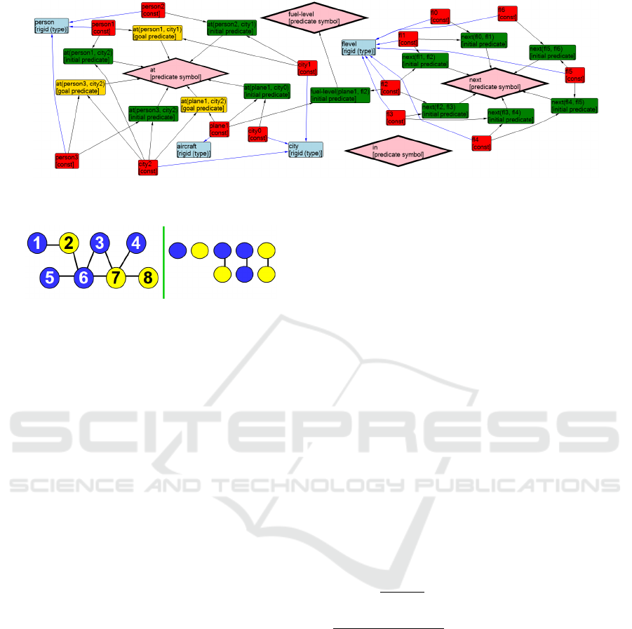
Figure 1: Example of an object graph for the initial state of problem pfile2 of the zenotravel domain.
Figure 2: Left-hand side: a simple graph used to demon-
strate computation of features. Right-hand side: a set of
graphs B
2
2
.
decomposed into a sequence of several atomic op-
erations of 3 types: AddVertex, RemoveVertex and
AddEdge. For example, in Zenotravel, there is an ac-
tion a = load(person1, city1, plane1). Given G(s),
we can construct G(γ(a, s)) by first removing ver-
tex that represents predicate at(person1, city1), then
adding vertex for predicate in(person1, plane1) and
then successively adding edges between the new ver-
tex and vertices for in, person1 and plane1.
Given graph G, its vertex v and a set of graphs B
q
,
we define contribution of a vertex v to F(G) denoted
by C(v) as a set of all occurrences of graphs from
B
q
in G which intersect with v. We will now show
how each of the three atomic operations can be per-
formed incrementally given G(s), F(s) and C(v) for
every vertex of G(s).
Remove Vertex: For each c ∈ C(v), remove c
from every C(v
i
) that contains it, decrease values in
F(s) accordingly. Remove v from G(s).
Add Vertex: Add v to G(s), add one new occur-
rence of a subgraph containing a single vertex with
the given label to C(v), increment the the correspond-
ing element of F(s).
Add Edge:
1. replace every occurrence c ∈ C(v
1
)∩C(v
2
) by oc-
currence of a graph with the same vertex set and
one more edge added at the corresponding loca-
tion.
2. for every occurrence c ∈ C(v
1
) \ C(v
2
) such that
|c| ≤ q − 1 create a new occurrence on vertices
c∪{v
2
}. If c contained some vertex adjacent to v
2
,
edges between these vertices and v
2
will be taken
into account when determining which graph from
B
q
occurred on c ∪ {v
2
}.
3. repeat the previous step symmetrically for v
2
, then
add the edge to G(s).
Using a carefully designed data structure, we can
perform AddVertex, RemoveVertex as well as the step
1 of AddEdge in time O (1), steps 2 and 3 can be
performed in time O (|C(v
1
)|) and O(|C(v
2
)|) respec-
tively.
5 ERROR FUNCTION FOR THE
TRAINING
We train the network by a standard gradient-descent
optimizer which iteratively updates parameters of the
network in order to minimize the given loss func-
tion. We are solving a regression task - predict-
ing a real number for each state. We experimented
with two loss functions: standard MSE defined as
MSE =
∑
(Y
i
−
ˆ
Y
i
)
2
n
and a MSE transformed by a log-
arithm (denoted LogMSE), defined as LogMSE =
∑
[log(Y
i
+1)−log(
ˆ
Y
i
+1)]
2
n
, where Y
i
is target of the i-th
sample (i.e., the real goal distance of the i-th state),
ˆ
Y
i
is output of the model on the i-th sample (i.e. the
value that would be used as a heuristic estimate for
the i-th state) and n is the number of samples. The
sum goes over all samples.
Figure 3 presents a histogram of fit of the trained
model when MSE is used. On the x-axis there is dif-
ference between target value and output, the height
of the column represents the number of samples that
fall into each category. Yellow columns show training
data, purple ones show test data. In Figure 4 we can
see accuracy of the model on samples with different
targets (blue columns). On the x-axis there is target
and the height of the column represents average of ab-
solute values of absolute error among all samples with
ICAART 2020 - 12th International Conference on Agents and Artificial Intelligence
84

corresponding target value. The model is well trained
having small error on both training and test data. The
use of MSE loss function leads to an even distribution
of the error among all samples regardless of their tar-
get (up to goal distance about 50). For example, the
model makes error of ±1.5 on states 50 steps from
goal, but makes about the same error (±1.5) also on
states that are 2 steps from goal.
Figure 3: Accuracy of the model. Yellow columns represent
training data, purple one represent test data.
During the deployment phase, however, the model
perform poorly. The heuristic is very accurate on
states far from goal, but our analysis showed that
making relatively large mistakes on states close to
goal hurts the performance a lot.
In order to improve the search efficiency, the ac-
curacy of the heuristic on states close to goal (i.e.
with target 0-10) needs to be much higher. This can
be achieved by using LogMSE as the loss function.
LogMSE minimizes the average of relative error, i.e.,
the ratio between target and output which enforces
low absolute error on samples close to goal and tol-
erates larger absolute error on samples further from
goal.
Figure 4: Absolute error on samples with different targets.
On the X-axis there is target - i.e. real goal distance, height
of the column shows average of absolute error (| Y
i
−
ˆ
Y
i
|)
over all samples that fall into that category. Blue color cor-
responds to network trained by MSE, orange to LogMSE.
Figure 4 illustrates this behavior as it compares
absolute and relative error on training and test sam-
ples for both loss functions. MSE (in blue) makes
large relative error on states close to goal while
LogMSE (orange) performs much better on these
states but has slightly larger error on states further
from goal. The total sum of error is similar for both
functions but its distribution with respect to the tar-
get is quite different. Experiments show that us-
ing LogMSE leads to better performance during the
search.
6 EXPERIMENTS
We conducted experiments on two standard bench-
mark domains: zenotravel and blocks because it is
easy to obtain training data for these domains. For the
purpose of the experiments, we implemented ad-hoc
solvers for the two domains and used them to gener-
ate training data. Our solvers are based on a genetic
algorithm combined with a greedy search, they are ca-
pable of solving most problems within a few seconds
and provide optimal or close-to-optimal solutions. We
test the method on 20 problems available for zeno-
travel
1
and the first 27 problems from blocks
2
.
For each problem P, we train the model using
the other problems from the domain (except P) as
the training data, and then use the trained model as
a heuristic with an A* algorithm to solve P. We com-
pare the quality of the resulting heuristic with the
Fast-Forward heuristic h
FF
(Hoffmann and Nebel,
2001). The heuristic has been around for quite some
time now but it is still often used as a baseline in ex-
periments, like in (H
¨
oller et al., 2019) for example.
The NN we used have 5 hidden layers with sizes of
(256, 512, 128, 64, 32) neurons respectively, and two
DropOut layers. We used ReLU activation function,
Xavier weight initialization and Adam as the training
algorithm (Goodfellow et al., 2016). The last layer
contained a single neuron with a linear activation to
compute the output. Architecture of the network was
chosen according to best practices for this kind of sce-
nario. The network is large enough to create efficient
representation of the data and drop-out layers prevent
overfitting. Similarly to other zero-learning scenar-
ios, the amount of time required for training is quite
high. For every problem, training the net took about 8
hours using over 1 million training samples for zeno-
travel and over 1.8 million for blocks.
We experimented with values of parameter q (size
of subgraphs) from 2 to 4. For values larger that
4, computing features of states is too costly and the
heuristic is not competitive. We experimented with
the two loss functions - MSE and LogMSE, and we
also tried to include value of the h
FF
among the fea-
tures of states. I.e., we first trained the network having
1
api.planning.domains/json/classical/problems/17
2
api.planning.domains/json/classical/problems/112
Deep Learning of Heuristics for Domain-independent Planning
85
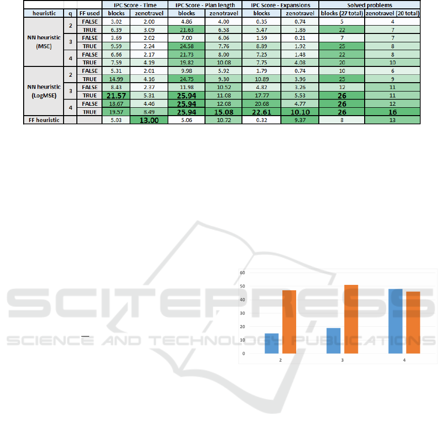
Figure 5: Results of experiments.
only the graph-based features as its inputs and then
another network that used both graph-based features
and h
FF
value of the state as its inputs. We conducted
experiments for all combinations of these parame-
ters: q ∈ {2, 3, 4}, lossFunction ∈ {MSE, LogMSE},
FFasFeature ∈ {true, f alse}. This gives us 12 differ-
ent neural net-based heuristics.
We used all 13 heuristics (12 NN-based + h
FF
) to
solve each of the problems. Search time was capped
at 30 minutes per problem instance. None of the
heuristic is admissible so they don’t guarantee finding
optimal plans. We compared performance of heuris-
tics using the IPC-Score. Given a search problem P,
a minimization criterion R (e.g. length of the plan)
and algorithms A
1
, A
2
, . . . , A
k
, the IPC-Score of A
i
on
problem P is computed as follows: IPC
R
(A
i
, P) = 0 if
A
i
didn’t solve P, or
R
∗
R
i
otherwise, where R
i
is value of
the criterion for the i-th algorithm and R
∗
= min
i
{R
i
}.
For every problem P, IPC
R
(A
i
, P) ∈ [0, 1] and higher
means better. We can then sum up the IPC-Score over
several problem instances to get accumulated results.
The IPC-Score takes into account both number of
problems solved as well as quality of solutions found.
We monitor four criteria: total number of problems
solved, IPC-Score of time, IPC-Score of plan length
and IPC-Score of number of expansions.
Figure 5 shows results for the two domains.
We can see that network trained by LogMSE is
superior to the one trained by MSE in all criteria on
both domains. As expected, higher values of q lead
to a more accurate heuristic: the number of expanded
nodes as well as plan length are better. The difference
is apparent especially for values 2 and 3. Using value
q = 4 still helps but computing features in this case is
slower and so A* expands less nodes per second and
overall results are not that much better than for q = 3.
Adding h
FF
as feature has a mixed effect. It is
very helpful on blocks domain when q ∈ {2, 3}, but
not much helpful when q = 4. See figure 6. This
indicates that subgraphs of size 2 and 3 cannot cap-
ture useful knowledge about a blocks problem hence
the network rely on h
FF
as the source of informa-
tion. Subgraphs of size 4 seem to be able to pro-
vide the required knowledge already and adding h
FF
doesn’t help anymore. This phenomenon is domain-
dependent and should be analyzed further in the fu-
ture. In general, adding h
FF
improves accuracy of the
NN so the resulting heuristic is more informed which
improves both number of expansions and plan length.
Due to the slow-down, though, adding h
FF
doesn’t
often improve number of problems solved.
Figure 6: Number of problems solved in blocks domain
(sum of both MSE and LogMSE). On the X-axis there is
q value, blue columns correspond to networks trained with-
out using h
FF
as feature, orange columns show networks
trained with h
FF
included.
Among the neural-based heuristics, the setting
with q = 4, h
FF
added and LogMSE performs best. If
we compare it with the h
FF
, we see that our method
vastly outperforms the baseline on blocks where it
solved 26 out of 27 problems while h
FF
can only
solve 8 problems. Even on problems solved by both
methods, the NN heuristic finds shorter plans and ex-
pands less nodes. On the zenotravel domain, our
method outperforms h
FF
in all criteria except Time.
As h
FF
can find suboptimal plans very quickly in
zenotravel, it is difficult to achieve better score even
though our method solved more problems within the
time limit.
ICAART 2020 - 12th International Conference on Agents and Artificial Intelligence
86

6.1 Performance Guarantees
The resulting heuristic is neither admissible nor ε-
admissible for any ε but we can still provide some the-
oretical guarantees of solution quality. We will only
provide here a simple bound and sketch of a proof.
Tighter bounds together with formal statements of
theorems and full proofs will be published in a sep-
arate paper.
Due to the stochastic nature of the NN-training al-
gorithm, output of the trained network on state s (de-
noted H(s)) must be considered a random variable.
Cost of the solution that A* finds with NN as heuris-
tic from state s (denoted A
H
(s)) is a random variable
as well. Assuming that ∀s
i
6= s
j
, H(s
i
) and H(s
j
) are
independent, we can state the following theorem.
Theorem 1. If for all states s: E[H(s)] = h
∗
(s), then
∀c > 1 : Prob[A
H
(s
0
) ≥ c ∗ (h
∗
(s
0
))
2
] <
1
c
Proof (sketch). Lets denote by Opt(s
0
) the optimal
path from s
0
to goal (a sequence of states). The
weighted A* efficiency theorem (Pearl, 1984) states
that
∀ε ≥ 1 : ∀s : h(s) ≤ ε ∗ h
∗
(s) ⇒ A
h
(s
0
) ≤ ε ∗ h
∗
(s
0
)
By a contraposition of the previous, we have
∀ε ≥ 1 : A
H
(s
0
) > ε ∗ h
∗
(s
0
) ⇒ (1)
∃s
i
∈ Opt(s
0
) : H(s
i
) > ε ∗ h
∗
(s
i
) (2)
hence
P[A
H
(s
0
) > ε ∗ h
∗
(s
0
)] ≤ (3)
P[∃s
i
∈ Opt(s
0
) : H(s
i
) > ε ∗ h
∗
(s
i
)] ≤ (4)
∑
s
i
∈Opt(s
0
)
P[H(s
i
) > ε ∗ h
∗
(s
i
)] (5)
(3) ≤ (4) comes from (1) ⇒ (2), while (4) ≤ (5)
can be achieved by applying Boole’s inequality which
states:
Lemma 2 (Boole’s inequality). Let A
i
be events, then
Prob[
S
A
i
] ≤
∑
Prob[A
i
]
Now, Markov’s inequality states that
∀s
i
: P[H(s
i
) ≥ ε ∗ h
∗
(s
i
)] ≤
E[H(s
i
)]
ε ∗ h
∗
(s
i
)
=
1
ε
(6)
By substituting (6) to (5) we get:
∑
s
i
∈Opt(s
0
)
P[H(s
i
) > ε ∗ h
∗
(s
i
)] ≤
∑
s
i
∈Opt(s
0
)
1
ε
=| Opt(s
0
) | ∗
1
ε
≤ h
∗
(s
0
) ∗
1
ε
Now for given c > 1, we set ε = c ∗ h
∗
(s
0
) which
gives us the required bound.
The proof works for planning without action costs,
i.e. where cost of every action is 1 but the theorem
still holds for planning with action costs.
We don’t require that all H(s
i
) are identically dis-
tributed. Assumptions of independence and unbiased-
ness of H(s
i
) can be justified by analyzing the bias-
variance tradeoff for NNs (Hastie et al., 2001). NNs
in general have high variance and low bias hence for
a large enough network, H(s) should be unbiased and
∀s
i
, s
j
: H(s
i
) and H(s
j
) should be close to indepen-
dent. Tighter bounds can be acquired if we take vari-
ance of H(s
i
) into account.
7 CONCLUSIONS & FUTURE
WORK
We presented a technique to automatically construct
a strong heuristic for a given planning domain. Our
technique is domain-independent and can extract
knowledge about any domain from a given set of
solved training problems without any assistance from
a human expert. The knowledge in represented by a
trained neural network.
We analyzed how the choice of loss function used
during the training affects performance of the learned
heuristic. We showed that the Mean Squared Error
– the most popular loss function – is not appropriate
for heuristic learning task and we presented a better
alternative.
We developed a novel technique for generating
features for states where we encode the state de-
scription directly without using existing heuristics.
The method allows to compute features incrementally
which is very useful in planning application. Our ap-
proach falls into category of zero-learning as it works
without any human-knowledge initially added. The
presented technique significantly outperforms a popu-
lar domain-independent heuristic h
FF
in both number
of problems solved and solution quality. We have also
provided a simple theoretical bound on solution qual-
ity when using learned heuristic, similar to bounds for
weighted A*.
As a future work, we will provide better bounds
on solution quality and conduct larger experiments on
Deep Learning of Heuristics for Domain-independent Planning
87

more domains to properly back the claims made in
this paper.
ACKNOWLEDGMENT
Research is supported by the Czech Science Founda-
tion under the project P103-18-07252S.
REFERENCES
Arfaee, S. J., Zilles, S., and Holte, R. C. (2010). Boot-
strap learning of heuristic functions. In Felner, A. and
Sturtevant, N. R., editors, Proceedings of the Third
Annual Symposium on Combinatorial Search, SOCS
2010. AAAI Press.
Arfaee, S. J., Zilles, S., and Holte, R. C. (2011). Learn-
ing heuristic functions for large state spaces. Artificial
Intelligence, 175(16).
Bisson, F., Larochelle, H., and Kabanza, F. (2015). Using a
recursive neural network to learn an agent’s decision
model for plan recognition. In Twenty-Fourth Interna-
tional Joint Conference on Artificial Intelligence.
Brunetto, R. and Trunda, O. (2017). Deep heuristic-learning
in the rubik’s cube domain: an experimental evalua-
tion. In Hlav
´
a
ˇ
cov
´
a, J., editor, Proceedings of the 17th
conference ITAT 2017, pages 57–64. CreateSpace In-
dependent Publishing Platform.
Cenamor, I., De La Rosa, T., and Fern
´
andez, F. (2013).
Learning predictive models to configure planning
portfolios. In Proceedings of the 4th workshop on
Planning and Learning (ICAPS-PAL 2013).
Chen, H.-C. and Wei, J.-D. (2011). Using neural networks
for evaluation in heuristic search algorithm. In AAAI.
Fink, M. (2007). Online learning of search heuristics. In
Artificial Intelligence and Statistics, pages 115–122.
Geissmann, C. (2015). Learning heuristic functions in clas-
sical planning. Master’s thesis, University of Basel,
Switzerland.
Goldberg, Y. (2017). Neural network methods for natural
language processing. Synthesis Lectures on Human
Language Technologies, 10(1):1–309.
Goodfellow, I., Bengio, Y., and Courville, A. (2016). Deep
Learning. MIT Press.
Groshev, E., Goldstein, M., et al. (2017). Learning gen-
eralized reactive policies using deep neural networks.
Symposium on Integrating Representation, Reason-
ing, Learning, and Execution for Goal Directed Au-
tonomy.
Groshev, E., Tamar, A., Goldstein, M., Srivastava, S., and
Abbeel, P. (2018). Learning generalized reactive poli-
cies using deep neural networks. In 2018 AAAI Spring
Symposium Series.
Hastie, T., Tibshirani, R., and Friedman, J. (2001). The
Elements of Statistical Learning. Springer Series in
Statistics. Springer New York Inc., New York, NY,
USA.
Hoffmann, J. and Nebel, B. (2001). The ff planning system:
Fast plan generation through heuristic search. Journal
of Artificial Intelligence Research, 14:253–302.
H
¨
oller, D., Bercher, P., Behnke, G., and Biundo, S. (2019).
On guiding search in htn planning with classical plan-
ning heuristics. IJCAI.
Jim
´
enez, S., De la Rosa, T., Fern
´
andez, S., Fern
´
andez, F.,
and Borrajo, D. (2012). A review of machine learning
for automated planning. The Knowledge Engineering
Review, 27(4):433–467.
Konidaris, G., Kaelbling, L. P., and Lozano-Perez, T.
(2018). From skills to symbols: Learning symbolic
representations for abstract high-level planning. Jour-
nal of Artificial Intelligence Research, 61.
Mart
´
ın, M. and Geffner, H. (2004). Learning generalized
policies from planning examples using concept lan-
guages. Applied Intelligence, 20(1):9–19.
Nau, D., Ghallab, M., and Traverso, P. (2004). Automated
Planning: Theory & Practice. Morgan Kaufmann
Publishers Inc., San Francisco, CA, USA.
Pearl, J. (1984). Heuristics: Intelligent Search Strategies
for Computer Problem Solving. The Addison-Wesley
Series in Artificial Intelligence. Addison-Wesley.
Samadi, M., Felner, A., and Schaeffer, J. (2008). Learning
from multiple heuristics. In Fox, D. and Gomes, C. P.,
editors, AAAI, pages 357–362. AAAI Press.
Takahashi, T., Sun, H., Tian, D., and Wang, Y. (2019).
Learning heuristic functions for mobile robot path
planning using deep neural networks. In Proceedings
of the International Conference on Automated Plan-
ning and Scheduling, volume 29, pages 764–772.
Thayer, J., Dionne, A., and Ruml, W. (2011). Learning
inadmissible heuristics during search. In Proceedings
of International Conference on Automated Planning
and Scheduling.
Yoon, S., Fern, A., and Givan, R. (2008). Learning control
knowledge for forward search planning. Journal of
Machine Learning Research, 9(Apr):683–718.
ICAART 2020 - 12th International Conference on Agents and Artificial Intelligence
88
