Enhancing Deep Spectral Super-resolution from RGB Images by

Enforcing the Metameric Constraint

Tarek Stiebel, Philipp Seltsam and Dorit Merhof

Institute of Imaging & Computer Vision, RWTH Aachen University, Germany

Keywords:

Spectral Reconstruction, Spectral Super-resolution, Metameric Spectral Super-resolution.

Abstract:

The task of spectral signal reconstruction from RGB images requires to solve a heavily underconstrained set of

equations. In recent work, deep learning has been applied to solve this inherently difﬁcult problem. Based on

a given training set of corresponding RGB images and spectral images, a neural network is trained to learn an

optimal end-to-end mapping. However, in such an approach no additional knowledge is incorporated into the

networks prediction. We propose and analyze methods for incorporating prior knowledge based on the idea,

that when reprojecting any reconstructed spectrum into the camera RGB space it must be (ideally) identical to

the originally measured camera signal. It is therefore enforced, that every reconstruction is at least a metamer

of the ideal spectrum with respect to the observed signal and observer. This is the one major constraint that

any reconstruction should fulﬁl to be physically plausible, but has been neglected so far.

1 INTRODUCTION

Spectral imaging has the advantage compared to RGB

imaging devices, that the acquired data contains more

accurate information on the spectral power distribu-

tion (SPD) of the light captured by the imaging de-

vice (spectral stimulus). This added information can

be useful for a broad variety of computer vision tasks

ranging from object detection and image classiﬁca-

tion to a more accurate color measurement. How-

ever, actually obtaining spectral images, even in the

reduced form of multi-spectral imaging, is still a com-

plicated task. An increased spectral resolution dur-

ing measurement comes at the cost of either a lim-

ited temporal resolution, e.g. ﬁlter wheel design

or spectral line scanning, or reduced spatial resolu-

tion, e.g. integrated devices based on macro pixels.

Therefore, alternative approaches have been devel-

oped. One possibility is to pursue a more computa-

tional approach by trying to compensate for an insuf-

ﬁcient measurement in form of a spectral reconstruc-

tion. The underlying idea is straight-forward: Since

it poses a severe challenge to acquire spectral images

directly, only capture images we can easily measure

instead: RGB images. Subsequently, compute the

missing information using adequate signal process-

ing techniques. However, this is an extremely under-

constrained problem.

While the task of recovering spectral images from

a low dimensional (e.g. RGB) spectral measurement

has been within the focus of distinct researchers for

decades (Hardeberg et al., 1999; Hill, 2002; Miyake

et al., 1999), it recently attracted novel attention, in

particular under the name of spectral super-resolution

and the application of deep learning (Arad et al.,

2018; Timofte et al., 2018). Prior to deep learning,

all approaches were more or less based upon the idea

of reducing the dimensionality of the spectral domain

utilizing proper basis functions. One comparably re-

cent example was proposed by Arad et al. (Arad and

Ben-Shahar, 2016) who learn a dictionary based map-

ping which was improved later on by Aeschbacher

et al. (Aeschbacher et al., 2017). The more mod-

ern solution is the application of deep learning, cur-

rently forming the state-of-the-art. A large variety

of approaches based on neural networks can directly

be taken from the 2018 NTIRE challenge on spec-

tral super-resolution (Arad et al., 2018). One of the

major advantages of convolutional neural networks

(CNNs) in particular is the fact, that they are capable

of implicitly incorporating contextual image informa-

tion (Stiebel et al., 2018). Instead of considering pix-

els individually, entire regions are processed and used

to reconstruct only a single SPD, not only leading to

a better performance in comparison to single pixel

based algorithms but also to an increased robustness

against noise. It is also possible to combine learned

basis functions with deep learning, as demonstrated

Stiebel, T., Seltsam, P. and Merhof, D.

Enhancing Deep Spectral Super-resolution from RGB Images by Enforcing the Metameric Constraint.

DOI: 10.5220/0008950100570066

In Proceedings of the 15th International Joint Conference on Computer Vision, Imaging and Computer Graphics Theory and Applications (VISIGRAPP 2020) - Volume 4: VISAPP, pages

57-66

ISBN: 978-989-758-402-2; ISSN: 2184-4321

by Jia et al. (Jia et al., 2017) or Nguyen et al. (Nguyen

et al., 2014). A rather novel approach has been pro-

posed by Kaya et al. (Kaya et al., 2018) who aim

at estimating a spectral image from an RGB image

taken under unknown settings. The approach consists

of a combination of neural networks for respectively

spectral sensitivity estimation from the combination

of an RGB image and a hyper-spectral image as well

as spectral super-resolution given knowledge of the

spectral sensitivity.

Deep learning based approaches usually require ex-

plicit knowledge of the spectral sensitivity function

of the imaging device. This way, a large training

set of corresponding pairs of RGB images and spec-

tral images can be generated from existing spectral

databases. Should the spectral sensitivity be unknown

and, instead, the training set be captured directly us-

ing paired spectral imaging and an RGB device, one

could argue that based on the paired images the spec-

tral sensitivity can be computed anyway. Follow-

ing the creation of the training data, a network (or

a combination of networks) is trained on the gener-

ated data to learn an end-to-end mapping from the

RGB to the spectral domain. However, no further

knowledge is considered, any mathematical or phys-

ical constraints have so far been completely ignored.

While spectral super-resolution is certainly not trivial,

there is one condition that always has to be fulﬁlled

and remains yet completely unchecked. There is the

metameric constraint that the spectral reconstruction

must be within the so-called metameric set. Every

spectral reconstruction must equal the actually mea-

sured camera signal when reprojected back into the

camera RGB space using the known camera sensitiv-

ity. Assuming knowledge of the spectral sensitivity,

this appears like an obvious choice for constraining

and therefore optimizing the reconstruction. The ex-

ploitation of metamerism was so far only considered

in more traditional approaches, which do not use deep

learning (Bianco, 2010).

The contribution of this work is adapting the neces-

sary theory regarding metamer sets (Finlayson and

Morovic, 2005) and proposing a modiﬁcation for any

deep neural network in order to enforce the metameric

constraint. A state of the art neural network to

describe the mapping from camera RGB-images to

spectral images is considered and exemplary modi-

ﬁed. The modiﬁcation is evaluated on an established

benchmark, the ICVL dataset (Arad and Ben-Shahar,

2016). The ICVL dataset does not only provide a

large hyper-spectral database, but it was also used

within the 2018 NTIRE challenge on spectral recon-

struction from RGB images (Timofte et al., 2018) and

therefore offers a valid comparison to a variety of al-

gorithms. It is demonstrated, how the incorporation of

the metameric constraint into the networks prediction

can increase the convergence properties during train-

ing. In the absence of noise, it also yields superior

results in contrast to the original approach. Last, an

analysis on the inﬂuence of noise is provided.

2 THEORETICAL FOUNDATION

We will start by summarizing the necessary un-

derlying theory regarding image formation and

metamerism. Assuming a q-dimensional imaging de-

vice, signal formation is modeled using

g = σ ·S

cam

· r, (1)

where r ∈ R

denotes a spectral stimulus that results

in the measured camera signal g ∈ R

when viewed

by a camera associated with the spectral sensitivity

cam

∈ R

q×k

. The scaling factor σ might be inter-

preted as exposure time and is used as normalization

to map general spectral stimuli onto a valid camera

signal range. We assume a spectral sampling rang-

ing from 400nm to 700nm in 10nm steps and only

consider RGB images for the remainder of this work,

resulting in q = 3 and k = 31.

The linear model described by Eq. 1 is on an ab-

stract level a projection of a 31 dimensional space

onto a three dimensional space. Due to the nature

of such a projection, there exists an inﬁnite amount

of distinct spectral stimuli which all project onto an

identical camera signal. All these stimuli are called

metamers with respect to the observed camera signal

as well as the camera sensitivity. The task of spectral

super-resolution amounts to ﬁnding a solution to the

inverse mapping of Eq. 1, i.e. predicting a 31 dimen-

sional signal based on the three dimensional signal,

which is an extremely ill-posed problem. Put differ-

ently, any stimulus that is a metamer is a viable solu-

tion.

It is well established, that a reconstructed spectral

stimulus can be separated into two parts: a particu-

lar solution , r

, and a metameric black solution, r

(Finlayson and Morovic, 2005),

r = r

+ r

. (2)

An open question to date is the appropriate way to

actually perform this separation. Since there are cer-

tain degrees of freedom involved, a unique separation

does not exist. However, the topic of an adequate ba-

sis is not the focus of this work. We will therefore

settle with the trivial approach to obtain a particular

solution by considering the Moore-Penrose inverse

= P · g, (3)

VISAPP 2020 - 15th International Conference on Computer Vision Theory and Applications

Network Architecture

RGB Image Spectral Image

(a) Original

Network Architecture

RGB Image Spectral Image

(b) Proposed Modiﬁcation

Figure 1: Proposed modiﬁcation to enforce the metameric constraint.

with

P = S

(SS

)

−1

∈ R

k×q

. (4)

The matrix P represents a q dimensional basis within

the spectral domain, forming a spectral subspace that

is directly observable by the camera. On the con-

trary, there is the subspace of all metameric blacks,

B ∈ R

k×(k−q)

, which is spanned by the null-space of

B = null(S). (5)

Since the basis of the metameric blacks is by deﬁni-

tion orthogonal to the camera sensitivity, any change

within this subspace remains hidden to the camera

0 = S · r

, (6)

thus the name.

3 METHODS TOWARDS

ENFORCING METAMERISM

In this section, we will propose different approaches

for deep learning based spectral reconstruction to con-

sider the metameric constraint in an explicit way.

3.1 Estimating Metameric Blacks

A mathematically enforcing approach is to shift from

directly predicting a spectral image based on an

RGB image to only predicting the position within the

metameric black space. Since the space of metameric

blacks is of dimension n = k − q = 28, the dimen-

sional complexity of signal prediction is reduced from

31 to 28, hopefully leading to an enhancement of the

Algorithm 1: Modiﬁcation.

1: procedure INITIALIZE

2: B = nullspace(S)

3: P = S

(SS

)

−1

4: network ← NeuralNetwork(n out = k − q))

5: procedure RECONSTRUCT(rgb img)

6: r

= B · network(rgb img)

7: r

= P · rgb img

8: r = r

+ r

9: return r

networks prediction capability. Additionally, any re-

construction achieved in such a way is by deﬁnition

guaranteed to be a metamer, since only the metameric

black is predicted by the network. The metameric

black may in turn be chosen arbitrarily, since it does

not effect the observed camera signal.

Original network architectures are designed to learn

an end-to-end mapping from RGB images towards

the 31 dimensional spectral images. In order to apply

the proposed modiﬁcation, the networks themselves

do not need to be changed. They still assume RGB

images as input, but the amount of output dimensions

is reduced from 31 to 28, i.e. any network now only

predicts the metameric blacks within the metameric

subspace with respect to the sensing device. The pre-

dicted metameric blacks are combined with the par-

ticular solution, r

, for each given camera signal ac-

cording to Eq. 2 and 4, resulting in the actual spectral

reconstruction. The necessary steps to modify the net-

works workﬂow are outlined in Al. 1 and visualized

in Figure 1.

3.2 Metameric Loss

As an alternative, a less strict possibility towards con-

sidering the metameric constraint on the spectral re-

construction is proposed in form of an extended loss

function. An additional term is introduced that is en-

tirely devoted to the metameric constraint. Instead of

only evaluating the spectral reconstruction, I

spec

, by

comparing it to the ground truth, I

spec

, using the error

metric M(·), e.g. RMSE, the spectral reconstruction is

additionally reprojected onto the camera signal space

using Eq. 1 and the known camera sensitivity func-

tion. The resulting reconstructed RGB image, I

rgb

can likewise be compared to the original input RGB

image, I

rgb

. Combining both parts together yields the

newly proposed total loss, L,

L = αM(I

rgb

, I

rgb

) + M(I

spec

, I

spec

), (7)

with α ∈ [0, ∞) denoting a linear weighting term on

the metameric constraint. An α-value of 0 corre-

sponds to a pure spectral loss with no change at all,

whereas a value of 1 corresponds to an equal weight-

ing of both the spectral and the metameric loss. The

metameric loss should always reach a value of zero,

if the spectral reconstruction is in fact a metamer. In

Enhancing Deep Spectral Super-resolution from RGB Images by Enforcing the Metameric Constraint

400 500 600 700

wavelength in nm

0.00

0.25

0.50

0.75

1.00

rel. sensitivity

(a) Kodak DCS 420

400 500 600 700

wavelength in nm

0.00

0.25

0.50

0.75

1.00

rel. sensitivity

(b) Nikon D1X

400 500 600 700

wavelength in nm

0.00

0.25

0.50

0.75

1.00

rel. sensitivity

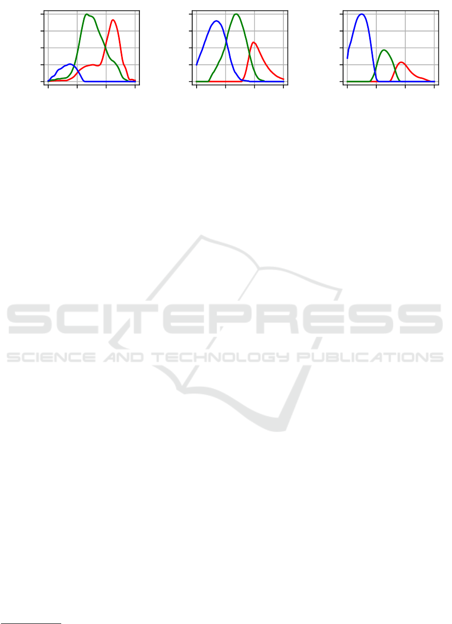
Figure 2: The relative spectral sensitivity functions of the considered RGB cameras (Kawakami et al., 2013).

reality, sources for inaccuracies like noise effects or

an imperfect measurement of the spectral sensitivity

function can be expected to ensure metameric loss

values greater than zero.

4 EXPERIMENTAL SETUP

In the following, the evaluation process of the pro-

posed methodologies as well as the precise steps taken

to generate the results are described.

4.1 Training Data

An extended version of the ICVL dataset (Arad and

Ben-Shahar, 2016) is considered, as it was published

during the 2018 CVPR Challenge on spectral recon-

struction (Timofte et al., 2018). The database forms

the largest freely available hyper-spectral database to

date. In summary, the training set consists of 256

spectral images mostly having a spatial resolution of

1392 x 1300, whereas there are 5 images within a

respective validation and test set. The spectral reso-

lution ranges from 400nm to 700nm in 10nm steps.

Based on a given camera sensitivity, all spectral im-

ages are projected into a cameras RGB signal space

using Eq. 1. A total of three different cameras are con-

sidered: Sony DXC 930, Kodak DCS 420 and Nikon

D1X. The associated spectral sensitivity functions are

publicly available (Kawakami et al., 2013). Their cor-

responding relative sensitivities are displayed in Fig-

ure 2.

Since the spectral images of the dataset are not nor-

malized in any way but provide the original light in-

tensities as captured in wild, all computed camera im-

ages need to be appropriately scaled. Such a scal-

ing must be performed for each of the three camera

models individually and might be interpreted as a real

cameras exposure time. Typical desired signal ranges

are [0, 1] or [0, 255]. In this work, the latter was

http://icvl.cs.bgu.ac.il/ntire-2018/

chosen. The reason is our interest in modeling the po-

tential effect of an 8bit signal encoding. In total, three

different signal scenarios were generated:

• Ideal

The calculated camera signals are used directly

in ﬂoating point precision for training and eval-

uation.

• Quantization

In order to consider a more realistic scenario,

quantization was applied to the ideal RGB images

assuming 8bit.

• Quantization & Noise

As a last scenario, the already quantized RGB

images were additionally disturbed using white

noise with a standard deviation of 1.

An open question is still the proper calculation

of the scaling factor. Within previous work, all im-

ages were typically scaled such that the maximal ob-

servable color signal equals the value 255 across the

entire dataset. Since such an approach of normaliz-

ing spectral data has been frequently followed and

already found a wide adaption especially within the

deep learning community, it is also considered within

this work. However, it comes with a couple of im-

portant underlying assumptions. In analogy to the

task of color constancy, which aims at estimating and

compensating the inﬂuence of an unknown illuminant

onto basically any image, the described approach of

normalizing spectral data can be seen a max-spectral

algorithm (Gijsenij et al., 2011). It is based on the un-

derlying idea, that at some arbitrary position within

an image, the light source is either directly observ-

able or through the reﬂection at a white surface. In

a Lambertian world, any object potentially reﬂecting

the emitted light is expected to not reﬂect more light

than the incident amount. The maximal observable

signal must therefore correspond to the light source.

A more reasonable approach for determining the scal-

ing factor might be the explicit consideration of a real

white reference. This is especially the case due to

the dataset actually containing images of white boards

VISAPP 2020 - 15th International Conference on Computer Vision Theory and Applications

0 50 100 150 200 250

signal value

0.0

0.2

0.4

0.6

0.8

1.0

relative frequency

(a) Histogram

0 50 100 150 200 250

signal value

0.0

0.2

0.4

0.6

0.8

1.0

cumulative density

(b) Cumulative histogram

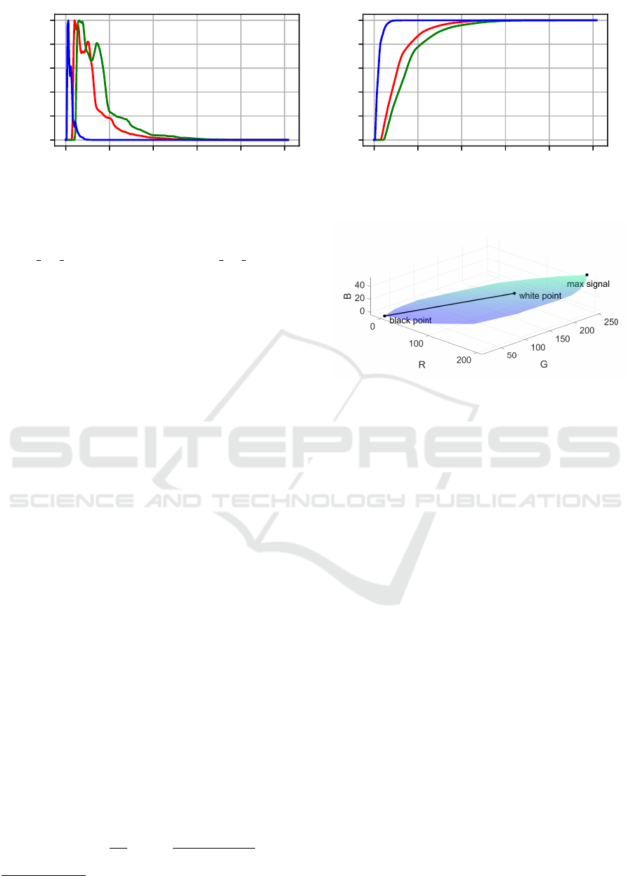
Figure 3: Histograms on the occurrences of camera signals across the entire dataset for the Kodak camera.

and calibration patterns. For example, image 26

(BGU HS 00026) and image 52 (BGU HS 00052) of

the dataset contain a white reference that can be used

for an estimate on the illuminant. The estimated SPD

of the illuminant is subsequently projected into cam-

era signal space to obtain its white point and used for

signal normalization. The normalization is achieved

by deducing a scaling factor such that the white point,

i.e. the projected illuminant, has at maximum a signal

value of 255. As an alternative approach to the max-

imum signal scaling, the white point based approach

is additionally followed for comparison.

4.2 Network and Training Details

Within this work, we restrict ourselves to the U-Net

based architecture proposed by Stiebel et al. (Stiebel

et al., 2018), because it is publicly available

and

therefore guarantees reproducibility. It was shown

to reach state-of-the-art performance for the task of

spectral reconstruction from RGB images (Timofte

et al., 2018) and thus ensures a fair comparison.

While we chose a single architecture for testing pur-

poses, all proposed steps can be applied to any archi-

tecture of choice in an analogous way. The network

is considered in its original version, which from now

on will be called the vanilla network, as well as in

a modiﬁed version containing our proposed changes

such that it only predicts the metameric blacks.

All training details were left untouched and are there-

fore identical to the original work (Stiebel et al.,

2018). In summary, every network is trained for 5

epochs using Adam optimization and a learning rate

of 0.0001 in any considered scenario. The batch size

is 10 with a patch size of 32. Both the spectral loss as

well as the metameric loss are computed by the mean

relative absolute error (MRAE),

MRAE(I, I

) =

∑

i=1

∑

j=1

I(i, j) − I

(i, j)

I(i, j)

|, (8)

https://github.com/tastiSaher/SpectralReconstruction

Figure 4: The set of all potential camera signals for the Ko-

dak camera.

with I denoting the ground truth image having m rows

and n columns and I

the reconstruction.

All implementations were carried out using Python

and Pytorch. The training process itself was run

on a single graphics card of the type NVIDIA GTX

2080TI.

5 RESULTS AND DISCUSSION

First of all, an analysis of the dataset itself is pro-

vided and the inﬂuence of a proper scaling factor is

discussed. Considering all the generated images for

the ideal scenario, a closer look is taken upon the dis-

tribution of all potential color signals across the entire

dataset. For starters, a scaling factor corresponding

to the maximum possible signal value is assumed. A

channel wise histogram analysis was conducted. The

results are exemplary visualized for the Kodak camera

in Fig 3. It is immediately visible that the majority of

color signals is within the lower half of the cameras’

dynamic range. Such an uneven data distribution is

not desirable and may lead to a bias in ﬁnal predic-

tion results. The distributions in case of the other two

camera devices turn out in an analogous way. This is

an issue that can be treated by choosing a scaling ac-

cording to a true white reference.

While all three camera channels are considered sepa-

Enhancing Deep Spectral Super-resolution from RGB Images by Enforcing the Metameric Constraint

Table 1: Resulting error metrics for both the vanilla network as well as the modiﬁed version only estimating the metameric

blacks. All camera images were scaled according to the maximal signal. The reported values represent the average results

over the test set.

Vanilla Network Metameric Blacks

MRAE RMSE GFC MRAE RMSE GFC

Ideal

Sony DXC 930 0.01677 23.75 0.99916 0.01542 23.96 0.99914

Kodak DCS 420 0.01325 17.08 0.99951 0.01298 16.37 0.99954

Nikon D1X 0.01416 19.84 0.99936 0.01412 19.26 0.99942

Quantization

Sony DXC 930 0.02316 28.18 0.99880 0.04674 41.73 0.99550

Kodak DCS 420 0.01722 17.87 0.99943 0.05400 60.74 0.99615

Nikon D1X 0.01745 18.42 0.99949 0.03130 28.73 0.99800

Quantization & Noise

Sony DXC 930 0.03007 31.73 0.99853 0.07857 74.51 0.98774

Kodak DCS 420 0.02426 20.33 0.99926 0.09700 127.2 0.97909

Nikon D1X 0.02317 22.86 0.99915 0.05518 50.65 0.99367

rately within the histogram analysis, their interaction

is also highly relevant. Of particular interest is the

3 dimensional subspace containing all possibly mea-

surable camera signals. It was estimated by comput-

ing the convex hull over all color signals within the

dataset. The resulting volume is depicted in Fig. 4.

Additionally, the white point as it is observable from

the white reference is explicitly marked in the visual-

ization. The black point is also highlighted for a bet-

ter understanding. The line passing through both the

black and white point might be considered as some

sort of lightness axis. In total, when considering a

scaling according to the white reference, more than

99% of all values were found to be still representable

without being subject to a potential signal clipping.

This is due to all pixels exceeding the white point

showing either dead pixels or local highly specular re-

ﬂections, both of which are limited in numbers. It will

be concluded that a proper scaling according to a true

white reference is advantageous. However, we will

continue using the maximum signal scaling variant,

since it is common practice within the deep learning

community.

5.1 Estimating Metameric Blacks

An extensive study was performed and is provided

to analyze the potential change in performance due

to the proposed network modiﬁcation. Tab. 1 dis-

plays the reconstruction results for both the vanilla

network and the modiﬁed version in case of all con-

sidered scenarios. For every permutation of network

setup, scenario and camera, the network is trained

from scratch upon the training set and evaluated over

the test set. Considered error metrics are the mean

relative absolute error as described by Eq. 8, the root

mean squared error (RMSE) and the goodness-of-ﬁt

coefﬁcient (GFC). A GFC value greater than 0.999

represents a good reconstruction and a value greater

than 0.9999 an excellent reconstruction (Imai et al.,

2002). The reported metrics in Tab. 1 are the com-

puted mean values over the test image set.

Different trends can be observed. The most intuitive

observation is an increasing reconstruction error with

the considered scenarios difﬁculty, i.e from ideal over

quantization to noisy. This is also independent of the

chosen camera model. The respective camera models

show differences in their performance relative to each

other. For most scenarios, the Kodak camera outper-

forms its contenders. The Nikon camera comes sec-

ond, with the Sony camera closing in last. These dif-

ferences in performance can be attributed to the dif-

ferences in the cameras spectral sensitivities. The best

ranking sensitivities of the Kodak device are probably

closer to some underlying basis function within the

considered spectral dataset and therefore able to cap-

ture more spectral information.

However, opposing trends become apparent when

comparing the metameric constraint network to its

vanilla version. The modiﬁed network always outper-

formed its original counterpart within the ideal set-

ting. Restraining the possible solution space by three

dimensions using the metameric constraint does in

fact help the network to reach better results. Ad-

ditionally, the modiﬁcation also has a positive inﬂu-

ence on the training process itself. Fig. 5 displays an

VISAPP 2020 - 15th International Conference on Computer Vision Theory and Applications

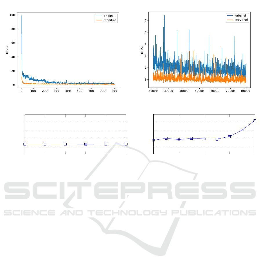
Figure 5: Exemplary training process for the original and modiﬁed network in an ideal world for the Kodak camera.

0 0.2 0.4

0.6

0.8 1

MRAE · 100

(a) Ideal

0 0.2 0.4

0.6

0.8

MRAE · 100

(b) Quantization

Figure 6: Evaluation of the metameric loss. The higher the value α, the more is the metameric loss term weighted.

exemplary loss function during the training for both

the modiﬁed network (orange) and the vanilla version

(blue). Particularly in the beginning, the inﬂuence of

the forced metameric constrained is signiﬁcant. Since

independent of the networks’ processing the recon-

structed spectra are forced to be at least metameric to

the true spectral stimulus, even the initial approxima-

tion is at least remotely close. This leads to a way

faster convergence due to the better initialization by

design. In total, the modiﬁed version converges ap-

proximately four times faster. Even providing an un-

limited amount of training time, the original network

is never able to reach the modiﬁed networks predic-

tive capabilities. This behavior is consistent for all

considered cameras and experiments we conducted,

showing great potential for physically motivated re-

strictions on a neural networks prediction.

However, the prediction results of the modiﬁed net-

work are actually worse than the vanilla version when

leaving the ideal world. The inﬂuence of disturbances

on the prediction is of great interest, since they can

most certainly be expected in a real world applica-

tion. Metamer based spectral reconstruction appears

to be rather sensitive in this regard. The networks’

predictive capability appears insufﬁcient to compen-

sate for noise effects, when limited by the metameric

constraint. This can be seen for both the quantized

and noisy scenario. In fact, the prediction quality sig-

niﬁcantly worsens with the added noise in comparison

to just quantization noise. The ﬁxed initial particular

solution based on a measured camera signal can most

likely be hold accountable for this effect. This way,

any disturbances contained within camera signals are

propagated and possibly enhanced, leading to initial

estimates on the particular solution that are too far off

and cannot be ﬁxed.

Finally, an interesting behavior can be observed for

the quantized and noisy scenario in conjunction with

the metameric constraint network. The relative per-

formance of the different camera devices to each other

changes. In fact, the ranking is almost inverted. The

originally best performing device, the Kodak camera,

achieves now the worst results. It demonstrates that

the choice of sensitivity is of great importance and

should always be optimized for the task at hand.

5.2 Modiﬁed Loss

As an alternative to the mathematically strict enforce-

ment of the metameric constraint, a modiﬁed loss was

proposed. It might be seen as weaker constraint hope-

fully placing less restrictions on the network to remain

Enhancing Deep Spectral Super-resolution from RGB Images by Enforcing the Metameric Constraint

1 2 3 4 5 6 7 8 9 10 11 12 13 14 15 16 17 18 19 20 21 22 23 24 25 26 27 28 29

position along lightness axis

100

150

200

250

MAE

(a) Reconstruction error within the spectral domain

1 2 3 4 5 6 7 8 9 10 11 12 13 14 15 16 17 18 19 20 21 22 23 24 25 26 27 28 29

position along lightness axis

0.0

0.2

0.4

0.6

0.8

1.0

MAE

(b) Reconstruction error within the RGB signal domain

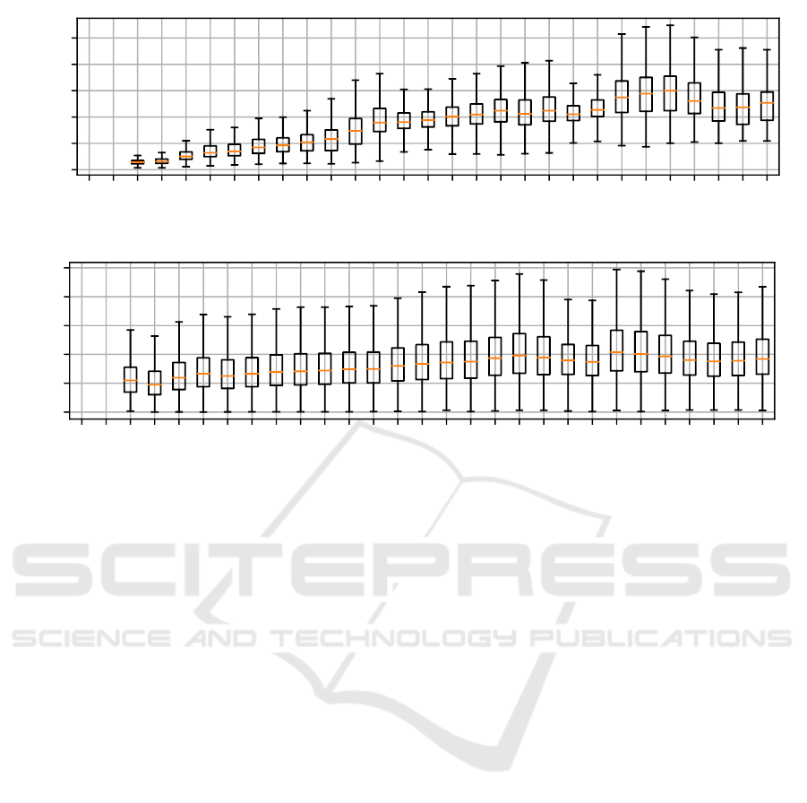
Figure 7: A visualization of the reconstruction error of the vanilla neural network as a box plot depending on the signal

position inside the OCS for the Kodak camera. A higher position on the lightness axis corresponds to a more centralized

signal position inside the OCS. For a better clariﬁcation, the lightness axis is explicitly visualized in Fig 4.

robust in the presence of noise. In analogy to the re-

sults presented in Tab. 1 the analysis was performed.

However, an additional parameter needs to be eval-

uated, the metameric loss weight α, as described by

Eq. 7. For a better understanding, the results were vi-

sually processed. The inﬂuence of the added loss is

exemplary visualized in Fig. 6 for both the ideal and

quantized scenario for the Kodak camera. In an ideal

world the added metameric term does not appear to

have any inﬂuence at all. When considering quantiza-

tion, it can be seen though, that an increasing term of

α, i.e. a higher weighted inﬂuence of the metameric

loss component, has a negative impact on the poten-

tial reconstruction of the network. In fact, an α-value

of 0 appears to be ideal, i.e. no metameric loss term

at all. This result is representative and consistent for

all experiments we conducted. When considering the

noisy scenario, the negative impact of the metameric

loss term also only increases. Like the proposed net-

work modiﬁcation, the metameric loss negatively im-

pacts the result in the presence of noise, but in contrast

to before, it neither has a positive impact in an ideal

world.

5.3 Vanilla Network

Explicitly considering metameric constraints showed

mixed effects on the potential prediction quality of

the neural network. While a signiﬁcant performance

increase within an ideal world was demonstrated,

the moment any disturbances as little as quantiza-

tion noise are introduced the added constraints seem

counter productive. In order to acquire a better under-

standing as to why, a closer look is taken upon the pre-

diction quality of the vanilla network. It is known that

the corresponding metameric set of a color signal is

the larger the more centralized a camera signal inside

the camera signal space becomes (Finlayson and Mo-

rovic, 2005). Therefore, the average prediction error

of the network is inspected depending on the corre-

sponding color signal position in its 3D signal space.

It can be expected that the more central a camera sig-

nal is located, the harder the reconstruction task be-

comes due to an increasing number of metamers and

therefore the worse the signal prediction gets. In order

to visualize the suspected behavior, every color signal

of the test image set is projected from its 3D signal

space as shown in Fig. 4 onto the lightness axis. The

original signal reconstruction error can then be eval-

uated depending on its relative position on the light-

ness axis. Simply speaking, the higher the position on

VISAPP 2020 - 15th International Conference on Computer Vision Theory and Applications

the lightness axis becomes, the more central the color

signal is located. The evolution of the spectral recon-

struction error over the lightness axis is displayed in

Fig. 7a as box plot. The considered error metric is

the mean absolute error (MAE), i.e. the average Eu-

clidean distance of the computed spectral reconstruc-

tion to its ground truth. A direct increase of the error

metric depending on the camera signal position is im-

mediately apparent.

Likewise to the proposed metameric loss, it is also

possible to project all spectral reconstructions back

into camera signal space and compare the result to the

input RGB image. When performing the same anal-

ysis as before but this time inside the camera signal

space, another trend is observed and shown in Fig. 7b.

In contrast to the spectral domain, the reconstruction

error remains rather constant independent of the po-

sition inside the signal space. It is worth highlighting

the average absolute error inside the camera signal do-

main. Since we are assuming an 8bit encoding and

therefore signals ranging from 0 to 255, the average

absolute errors are in fact in the same range as po-

tential quantization noise. One might argue, that the

reconstruction itself is already close to ideal. Any ad-

ditionally introduced reconstruction error within the

spectral domain must thus be along dimensions that

are not observable by the camera system. Therefore,

the limits of spectral reconstruction from RGB image

acquisition appear to be already reached. The map-

ping from one camera signal to many possible spec-

tral signals cannot be easily solved and most likely

only be further optimized in a signiﬁcant way by em-

ploying multi-spectral imaging. The interesting re-

sult though is, that the neural network appears to

be already capable of implicitly learning the realm

of metameric blacks itself. Made reconstruction er-

rors are mostly introduced in a meaningful way along

spectral dimensions no information is available on.

For further research, it would be highly interesting to

understand how and in what form the network actu-

ally represents the information.

6 CONCLUSION

Within this work, a modiﬁcation to neural networks

which perform the task of spectral reconstruction

from camera images was proposed. The modiﬁcation

is based upon the idea to mathematically enforce the

reconstruction to be at least within the metameric sub-

set of spectral stimuli to the true stimulus. The poten-

tial positive impact of the modiﬁcation was demon-

strated by applying it to a state-of-the-art model and

using it to reconstruct spectral images from differ-

ent simulated RGB cameras. Since the enforced

metameric constraint directly corresponds to a better

initialization, the training process also converges sig-

niﬁcantly faster. However, above ﬁndings only hold

true in an ideal world. The metameric based recon-

struction was found to be highly sensitive to noise,

probably preventing an application in the real world.

It was further demonstrated, that a consideration of

metamerism within the loss function does not yield

any positive effects at all. The reason is that knowl-

edge of a cameras’ sensitivity can already be success-

fully learned by directly training a neural network to

learn an end-to-end mapping from the camera signal

space to the spectral domain. As shown within this

work, such self-learned knowledge must be contained

somewhere within a fully trained network. However,

it is unclear in what form, leaving the potential extrac-

tion of a learned camera sensitivity from the network

as an interesting topic for further research.

REFERENCES

Aeschbacher, J., Wu, J., and Timofte, R. (2017). In de-

fense of shallow learned spectral reconstruction from

rgb images. 2017 IEEE International Conference on

Computer Vision Workshops (ICCVW), pages 471–

479.

Arad, B. and Ben-Shahar, O. (2016). Sparse recovery of

hyperspectral signal from natural rgb images. In Eu-

ropean Conference on Computer Vision, pages 19–34.

Springer.

Arad, B., Ben-Shahar, O., Timofte, R., Van Gool, L., Zhang,

L., Yang, M.-H., et al. (2018). Ntire 2018 challenge on

spectral reconstruction from rgb images. In The IEEE

Conference on Computer Vision and Pattern Recogni-

tion (CVPR) Workshops.

Bianco, S. (2010). Reﬂectance spectra recovery from tris-

timulus values by adaptive estimation with metameric

shape correction. J. Opt. Soc. Am. A, 27(8):1868–

1877.

Finlayson, G. D. and Morovic, P. (2005). Metamer sets. J.

Opt. Soc. Am. A, 22(5):810–819.

Gijsenij, A., Gevers, T., and van de Weijer, J. (2011). Com-

putational color constancy: Survey and experiments.

IEEE Transactions on Image Processing, 20:2475–

2489.

Hardeberg, J. Y., Schmitt, F. J. M., and Brettel, H. (1999).

Multispectral image capture using a tunable ﬁlter. In

Proc.SPIE, volume 3963, pages 3963 – 3963 – 12.

Hill, B. (2002). Optimization of total multispectral imag-

ing systems: best spectral match versus least observer

metamerism. In 9th Congress of the International

Colour Association, volume 4421, pages 481–486.

Imai, F. H., Rosen, M. R., and Berns, R. S. (2002). Com-

parative study of metrics for spectral match quality.

In Conference on Colour in Graphics, Imaging, and

Vision (CGIV), pages 492–496.

Enhancing Deep Spectral Super-resolution from RGB Images by Enforcing the Metameric Constraint

Jia, Y., Zheng, Y., Gu, L., Subpa-Asa, A., Lam, A., Sato, Y.,

and Sato, I. (2017). From rgb to spectrum for natural

scenes via manifold-based mapping. In International

Conference on Computer Vision (ICCV), pages 4715–

4723.

Kawakami, R., Hongxun, Z., Tan, R. T., and Ikeuchi, K.

(2013). Camera spectral sensitivity and white balance

estimation from sky images. International Journal of

Computer Vision.

Kaya, B., Can, Y. B., and Timofte, R. (2018). Towards

spectral estimation from a single RGB image in the

wild. CoRR, abs/1812.00805.

Miyake, Y., Yokoyama, Y., Tsumura, N., Haneishi, H.,

Miyata, K., and Hayashi, J. (1999). Development

of multiband color imaging systems for recordings of

art paintings. In Color Imaging: Device-Independent

Color, Color Hardcopy, and Graphic Arts.

Nguyen, R. M. H., Prasad, D. K., and Brown, M. S. (2014).

Training-based spectral reconstruction from a single

rgb image. In European Conference on Computer Vi-

sion (ECCV), pages 186–201. Springer.

Stiebel, T., Koppers, S., Seltsam, P., and Merhof, D. (2018).

Reconstructing spectral images from rgb-images us-

ing a convolutional neural network. In The IEEE Con-

ference on Computer Vision and Pattern Recognition

(CVPR) Workshops.

Timofte, R., Gu, S., Wu, J., Van Gool, L., Zhang, L., Yang,

M.-H., et al. (2018). Ntire 2018 challenge on sin-

gle image super-resolution: Methods and results. In

The IEEE Conference on Computer Vision and Pat-

tern Recognition (CVPR) Workshops.

VISAPP 2020 - 15th International Conference on Computer Vision Theory and Applications