
Automated 3D Labelling of Fibroblasts and Endothelial Cells in
SEM-Imaged Placenta using Deep Learning
Benita S. Mackay
1a
, Sophie Blundell
2
, Olivia Etter
3
, Yunhui Xie
1
, Michael D. T. McDonnel
1
,
Matthew Praeger
1
, James Grant-Jacob
1b
, Robert Eason
1c
, Rohan Lewis
3d
and Ben Mills
1e
1
Optoelectronics Research Centre, University of Southampton, Southampton, U.K.
2
Faculty of Engineering and Physical Sciences, University of Southampton, Southampton, U.K.
3
Faculty of Medicine, University of Southampton, Southampton, U.K.
Keywords: 3D Image Processing, Deep Learning, SBFSEM Images, Placenta.
Abstract: Analysis of fibroblasts within placenta is necessary for research into placental growth-factors, which are
linked to lifelong health and chronic disease risk. 2D analysis of fibroblasts can be challenging due to the
variation and complexity of their structure. 3D imaging can provide important visualisation, but the images
produced are extremely labour intensive to construct because of the extensive manual processing required.
Machine learning can be used to automate the labelling process for faster 3D analysis. Here, a deep neural
network is trained to label a fibroblast from serial block face scanning electron microscopy (SBFSEM)
placental imaging.
1 INTRODUCTION
The placenta is the interface between the mother and
the fetus mediating the transfer of nutrients while
acting as a barrier to the transfer of toxic molecules.
Poor placental function can impair foetal growth and
development and affect an individual’s health across
the life course (Palaiologou, et al., 2019). Serial
block-face scanning electron microscopy (SBFSEM)
has emerged as an important tool revealing the
nanoscale structure of the placenta in three-
dimensions. While this technique is revealing novel
structures, as well as the spatial relationships between
cells, it is limited by the time it takes to manually label
the structures of interest in hundreds of serial
sections. Developing a machine learning-based
approach would dramatically speed up this process
and enable more quantitative analytical approaches.
Here, a deep neural network is trained on stacks
of unlabelled, and their associated labelled, images of
a fibroblast within placental tissue. The neural
network is subsequently used to generate labels on
a
https://orcid.org/0000-0003-2050-8912
b
https://orcid.org/0000-0002-4270-4247
c
https://orcid.org/0000-0001-9704-2204
d
https://orcid.org/0000-0003-4044-9104
e
https://orcid.org/0000-0002-1784-1012
unlabelled images that were not used during training.
Visual comparison between the automated labelling
achieved via the neural network and manual labelling
of the fibroblast shows excellent agreement, with
quantitative analysis showing high pixel-to-pixel
comparison accuracy. This machine learning
approach also enables the labelling of different
structures, in this case endothelial cells within the
placenta, with the future possibility of other cell and
tissue types, such as osteoblasts within bone.
2 BACKGROUND
The study of fibroblasts in the placenta is necessary
for research in placental growth and development.
Fibroblasts can be found alongside mesenchymal and
mesenchymal-derived cells within the placenta
villous core stroma, between trophoblasts and fetal
vessels. Fibroblasts maintain the extracellular matrix,
the scaffold on which the blood vessels grow and on
which the trophoblast barrier lives. Trophoblast
46
Mackay, B., Blundell, S., Etter, O., Xie, Y., McDonnel, M., Praeger, M., Grant-Jacob, J., Eason, R., Lewis, R. and Mills, B.
Automated 3D Labelling of Fibroblasts and Endothelial Cells in SEM-Imaged Placenta using Deep Learning.
DOI: 10.5220/0008949700460053
In Proceedings of the 13th International Joint Conference on Biomedical Engineering Systems and Technologies (BIOSTEC 2020) - Volume 2: BIOIMAGING, pages 46-53
ISBN: 978-989-758-398-8; ISSN: 2184-4305
Copyright
c
2022 by SCITEPRESS – Science and Technology Publications, Lda. All rights reserved
number and function affects placental development
and function over the course of pregnancy,
influencing lifelong health and risk of chronic disease
in later life (Wang & Zhao, 2010) (Lewis, Cleal, &
Hanson, 2012).
3D images of placentas with nanoscale resolution
can be obtained through labelling of serial block face
scanning electron microscopy (SBFSEM) images
(Denk & Horstmann, 2004). Due to the number of
programmatical rules that would be required,
alongside limited contrast achievable in SBFSEM
imaging of placenta villi and multiple contextual
parameters, simple computer automation of labelling
has not yet been achieved, and all 2D images that
make up the larger 3D block must be manually
labelled. Conventional image segmentation for 3D
medical image data and techniques such as fuzzy
binarization can be combined to extract important
details from images and reconstruct into 3D models,
yet these approaches require intensive data
processing and a contrast/distinction in features,
which can be difficult to obtain in SBFSEM images
of tissue, and data loss from, for example,
binarization techniques can result in lower resolution
(Zachow, Zilske, & Hege, 2007) (Pugin &
Zhiznyakov, 2007). As the z-spacing between 2D
images represent the z-axis resolution in 3D, typically
30-100 nm, a typical 3D dataset will include hundreds
to thousands of individual images. In general, the
complexity of the labelling process and the pure
number of pixels (~109 pixels for this dataset) can
lead to a dedicated expert requiring weeks to months
to label an entire stack of 2D images.
However, as shown here, this challenge can be
solved via a neural network that is trained to
automatically label fibroblasts in SBFSEM images of
placentas.
We have recently shown that neural networks can
be effective at a wide variety of image processing and
image labelling processes for enhancing microscopy
resolution (Grant-Jacob, et al., 2019). The versatility
of deep learning has also resulted in computer-aided
diagnosis in the thorax and colon (Suzuki, 2013), the
liver (Chen, et al., 2013), the breast (Shan, Kaisar
Alam, Garra, Zhang, & Ahmed, 2016) and for
diseases such as Alzheimer’s (Yamashita, et al.,
2013). Here, we apply this technique, for the
automated labelling of fibroblasts in SBFSEM
images of placentas.
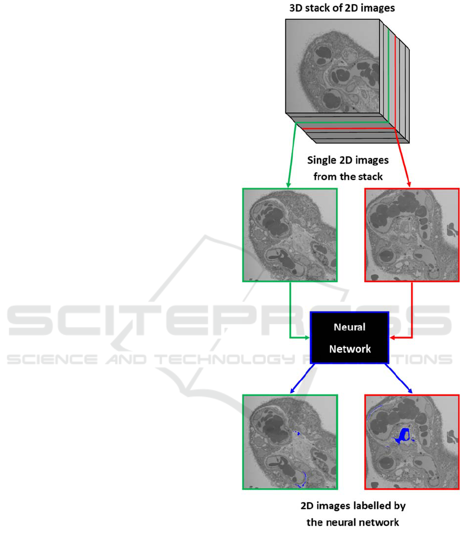
As shown in Figure 1, the purpose of this work is
to automate the labelling of fibroblasts across all 2D
SEM images in a 3D stack (943 in total). Automation
requires training a neural network to label the z-stack
images
without
human
involvement,
such
that
the
Figure 1: A 3D image consists of a stack of multiple 2D
SEM images, which can then be automatically labelled by
a neural network, which saves months of dedicated time in
manual labelling.
labels can then be isolated and converted using
standard imaging software into 3D projections
without requiring months of image processing.
Automated 3D Labelling of Fibroblasts and Endothelial Cells in SEM-Imaged Placenta using Deep Learning
47
3 METHOD
SBFSEM produces a series of high-resolution images
taken at sequentially deeper depths into a sample
which allow its internal structure to be revealed in
three-dimensions. This is achieved by placing an
ultramicrotome inside a scanning electron
microscope. The microscope creates an image of the
top of the sample (the block face), and the microtome
then cuts a thin layer (typically 50 nm) off the surface
of the sample allowing the next image to be taken
further into the tissue. This process is then repeated to
create hundreds or thousands of aligned images.
The deep neural network architecture for
transforming a 2D SEM image into a labelled image
is a variant designed specifically for image-to-image
translation and henceforth referred to as the network
(Isola, Zhue, Zhou, & Efros, 2018). The 3D image
consists of 943 images recorded at different z-
positions, which are named 001-943. All even
numbered images are extracted, not used for training
the network, and are instead used for testing the
effectiveness of the network for the labelling of
unseen images.
The network operates at a resolution of 256 by
256 pixels, so images are reduced via randomised
cropping from 2000 by 2000 to 512 by 512 before
being resized to 256 by 256. It is trained for 100
epochs (where one epoch is defined as training on all
training images exactly once, and one iteration is
defined as training on a single image) with a learning
rate of 0.001 and a batch size of 1, which takes
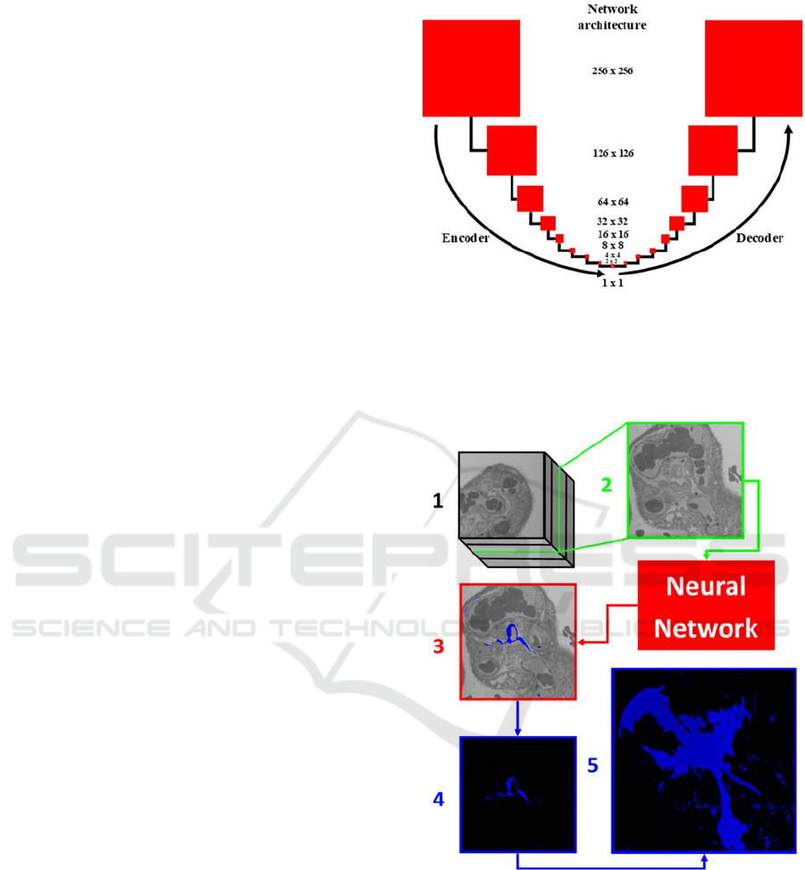
approximately 6 hours. The network is based on an
encoder-decoder architecture, with 17 layers, and
stride of 2, a 4 by 4 kernel size, and uses rectified
linear unit activation functions. This results in image
size decreasing from 256 by 256 down to 1 by 1, then
increasing back up to 256 by 256, as seen in Figure 2.
The encoder-decoder is based on a U-net structure
(Ronneberger, Fischer, & Brox, 2015), with skip
connections between the mirrored layers. The
discriminator is formed of 4 layers of convolutional
processes with stride of 2, taking the image size from
256 by 256 down to 32 by 32, leading to a single
output, via a sigmoid activation function that labelled
realistic or unrealistic. This architecture was chosen
instead of a simpler convolutional neural network,
typically used for image processing, as it can produce
high resolution output images and train on relatively
small datasets (Heath, et al., 2018).
After a training iteration, outputs from the
network are compared to real labelled images, leading
to network improvements achieved via
backpropagation. Figure 3 is an example of the whole
Figure 2: A block diagram of the network architecture used
for labelling SBFSEM images. Based on a U-Net encoder-
decoder framework, the image is downsized through
convolutional layers until it is 1 x 1 before being resized to
the original 256 x 256 input dimensions.
Figure 3: The automation process from stack image to 3D
projection. From the 3D stack (1), an unlabelled 2D SEM
image of the placenta (2) is input into the network. These
2D images are then labelled by the network (3). Here, an
image from the near the middle of the stack, 452, is labelled
blue where a fibroblast is present. The label is then
extracted from the rest of the image (4) so that all labels can
be collectively z-projected into a 3D image of a whole
fibroblast, where the z-axis is perpendicular to the page (5).
automation process. The input image, 2, is a 2D
section of the larger 3D stack, 3 is an automated
BIOIMAGING 2020 - 7th International Conference on Bioimaging
48
labelled image and 4 is the extracted label without
surrounding tissue imaged. This extracted label
image, alongside all others in the z-stack, is then
collectively computationally projected with readily-
available software (ImageJ) to produce a full 3D
model of the labelled fibroblast structure.
4 RESULTS
After the network is trained on odd numbered images,
the extracted unseen even numbered images are used
for testing the network. For error calculation, a pixel
is considered correct if the value in each position of
the network output image exactly matches the pixel
value in the corresponding position of the real
labelled image. A pixel difference of only ±1 (or
greater) in any of the three colour channels, out of a
standard 0-255 value range, is considered incorrect.
This is because a pixel is extracted as a label if it has
the exact value [0,0,255] at any position in the three
channel image, the blue colour seen in 4 and 5 of
Figure 5. The images used in analysis are sixteen 256
by 256 network output images combined to form a
single 1000 by 1000 image, where resolution is
limited by the GPU size available.
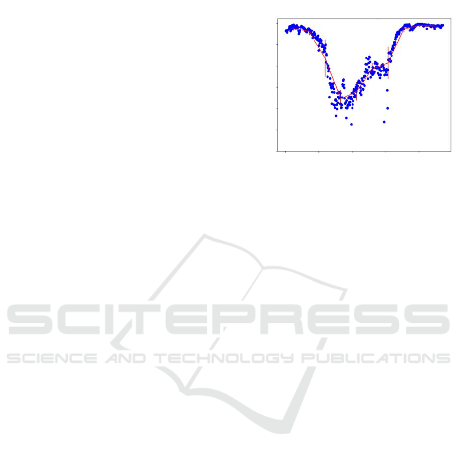
The error is graphically depicted as a percentage,
seen in Figure 4, and displayed visually, as seen in
Figure 5. In regions close to the beginning and end of
the stack, roughly positions up to 100 and then those
over 700, the error is less than 0.1%. This is due to
there being no labelled fibroblast in this region, which
is easier for the network to determine. This explains
why the error is largest in the central region around
position 300, where the labelled section is at its
largest. There is a larger boarder region around larger
labelled areas, and it is in this region where there is
most error. This is due to slight imperfections in the
training data, where manual labelling has been less
accurate around the edges of the fibroblast. This is
due to the amount of time manual labelling takes,
accuracy has been sacrificed in return for speed, and
also the limitations of human labelling; the human
eye cannot manage to contrast individual pixels at a
standard screen resolution, nor easily label at this
resolution with a standard computer mouse.
However, this does not result in areas with no
fibroblast to label being perfectly unlabelled by the
network. While there are areas of 0% error, there are
small fluctuations. This is due to there being only one
labelled fibroblast in the training data, yet more than
one fibroblast in the 3D stack. This conflicting data
leads to confusion within the network and therefore
an
amount of error is unavoidable. While the
Figure 4: Blue markers show the percentage of correct
pixels, where a pixel value of the network labelled image
matches the pixel value of the real labelled image, at the
position of the 2D image within the 3D stack for each tested
image. The red line is the mean and standard deviation
across every 10% of images.
percentage of incorrectly labelled pixels is never
greater than 1%, showing the promise of this labelling
technique, this confusion is easier seen when the two
types of errors, falsely not labelling where the
network should have labelled (false negative) and
falsely labelling where it should not have labelled
(false positive), are seperated.
The vast majority of errors come from fasle
negatives. In contrast, false positives occur in roughly
less than 0.2% of unlabelled pixels. The central
region has the lowerst percentage of false negatives
as the changes of other fibroblasts being in this region
dominated by the labelled fibroblast are smaller.
Even though a value of [0,0,254] would not be
distinguishable from [0,0,255] to the human eye, only
pixels with the value [0,0,255] are extracted as labels.
To more easily visualise the pixel error in labelling, a
coloured error image is created for each of the tested
z-stack images, seen in Figure 4. Blue pixels show the
correctly labelled pixels, red pixels show false
negatives (the network incorrectly did not label a
pixel), green pixels show false positives (the network
incorrectly labelled a pixel), and black pixels show
correctly unlabelled areas.
Differences between column 2 and 3 are difficult
to see clearly, and the vast majority of column 4
pixels are blue and black, which are the colours for no
error. The large amount of black, correct negative,
pixels is the reason that the overall error for the
network is so low (less than 1% error). The majority
of green pixels, false positives, are in regions
surrounding labelled fibroblast, which could be down
to
uncertainty in the network and inaccuracies in
100
99.9
99.8
99.7
99.6
99.5
0 200 400 600 800
Error in Testin
g
Data
Total Correct Pixels
(
%
)
Automated 3D Labelling of Fibroblasts and Endothelial Cells in SEM-Imaged Placenta using Deep Learning
49
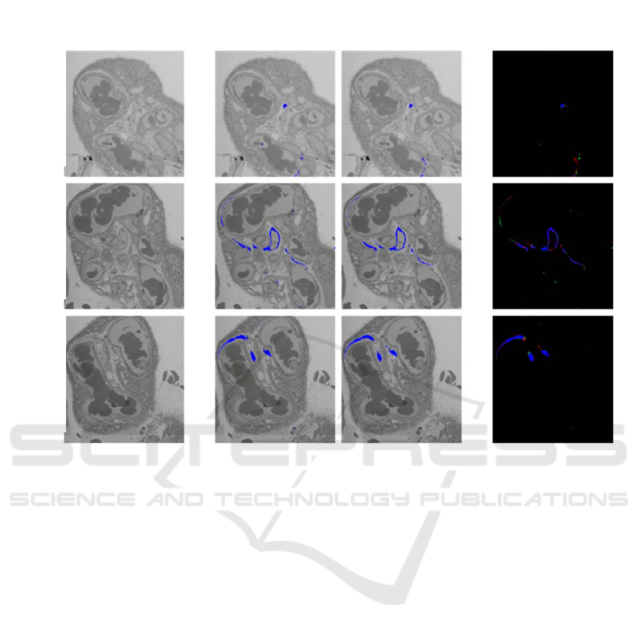
Figure 5: A visual error analysis for three positions within the stack, where A is frame 200, B is frame 400 and C is frame
600. The first column is the input for the network, an unlabelled z-stack image; the second is the output from the network, a
network labelled fibroblast; the third is the manually labelled fibroblast and the fourth column is a comparison between
columns 2 and 3, where black is correctly negative, blue is correctly positive, red pixels are falsely negative and green are
false positives.
human labelling. The red pixels, false negatives, are
similarly placed. This shows that, with the network
matching 99% of manual labelling, the correct shape
of the fibroblast is being labelled and provides the
vital information required for a 3D model.
5 ALTERNATIVE CELL TYPE
AND ALTERNATIVE SAMPLE
The labelling of endothelial cells requires a very
small adaption to the fibroblast labelling. A similar
network is used for endothelial labelling, which is
also based on an encoder-decoder architecture, with a
stride of 2, a 4 by 4 kernel size, and it uses rectified
linear unit activation functions. However, it has
double the number of layers, with 34 in total. This
results in image size decreasing from 256 by 256
down to 1 by 1, then increasing back up to 256 by
256, and then this resizing process is repeated.
Increasing the number of layers improves the
accuracy of the network labelling and the ability to
apply labelling to unseen samples. Unlike increasing
filter numbers, this did not present an increase in
necessary GPU size requirements in comparison to
previous network architecture.
The labelled endothelial data is also split in a
similar way to the previous fibroblast data. Odd
images within the range 001-327 are used for training
the network and even images in the same range are
used for testing. However, the range 328-367, both
odd and even, is also extracted for additional testing,
to make sure the network could extrapolate in areas
of the stack beyond that which it has already seen.
The images used in analysis are thirty-six 256 by
256 network output images combined to form a single
1500 by 1500 image, where resolution is once limited
by the GPU size available. By using a larger number
of 256 by 256 images, the resolution can be increased
without larger GPUs being required.
Input Ima
g
e
Network
Generated
Manuall
y
Generated
Visual
Com
p
arison
A
B
C
BIOIMAGING 2020 - 7th International Conference on Bioimaging
50
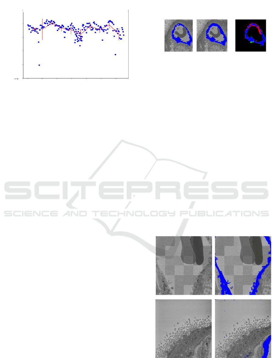
Figure 6: A graph of correct pixels as a percentage of total
pixels within the images vs the position of each image
within the stack. Blue markers show the percentage of
correct pixels, where a pixel value of the network labelled
image matches the pixel value of the real labelled image, at
the position of the 2D image within the 3D stack for each
tested image. The red line is the mean and standard
deviation across every 10% of images.
The network is trained on this stack for 50 epochs
before initial testing. Initial results for the automated
labelling of endothelial cells by a neural network are
extremely promising, with an accuracy of above 95%
for all unseen even numbered test images and images
within the range 158-187, which were also extracted
from the training data, as seen in Figure 6.
The mean pixel accuracy is between 98% and
99% for all images across the stack, with a slight dip
in the centre and towards the end of the stack. A drop
in accuracy towards the end of the stack (mean
accuracy of 98%) is due to the increase in labelled
areas compared to unlabelled areas and, as with
fibroblast labelling, the majority of error is in these
regions due to, for example, manual labelling error.
The central drop (mean accuracy of 98%) matches the
region of extracted images, 158-187. This dense
extraction of images provides an area where the
network has not seen similarly labelled images, as the
closest similar image is ± 15 images either side. The
mean error dropped by less than 1% for this region
compared to surrounding regions, showing that
labelling only every 1 in 15 images, rather than 1 in
2, would not impact the training and accuracy of the
network severely. New stacks introduced to the
training data in the future will therefore start at 1 in
every 10 images, as this will not overly impair chances
of correctly labelling the new stack. When the image
with the largest error of 4%, frame 40, is visually
analysed, as seen in Figure 7, it appears that the
network has incorrectly missed a large section of
labelled area, which is seen by the large area of red in
column 3. However, the network has correctly labelled
Figure 7: A visual comparison of automated labelling error
in frame 40, the frame with the highest error among the test
frames of this stack. Column 1 is the labelled output from
the network, column 2 is the manually labelled image and
column 3 is the difference between column 1 and 2, where
black pixels are correctly unlabelled, blue pixels are
correctly labelled, red pixels are falsely unlabelled and
green pixels are falsely labelled areas.
the endothelial cells and the manual labelling has
been rough and inaccurate in that region: automation
has outperformed manual labelling. As the network is
trained from manually labelled data, the maximum
prediction accuracy is therefore only limited by the
average accuracy of manually labelled training data.
To see how well the network can label data more
varied from the training data, an unlabelled image 40
frames away from the last seen training image
position (the last image in the stack) and a frame from
a completely unseen stack have been input to the
network, as seen in Figure 8. The labelling produced
by the network can be seen in. This is a manually
unlabelled area of the previously seen stack and a
different
unlabelled stack, so no comparison is
Figure 8: The output of and unseen region and an unseen
stack from the network. The first column is the input to the
network, while the second is the labelled output.
100
99
98
97
96
95
0 50 100 150 200 250 300
Error in Testing Data
Total Correct Pixels
(
%
)
40
Network
Generate
Manually
Generate
Visual
Comparison
Input Image
Network
Unseen Region
Unseen Stack
Automated 3D Labelling of Fibroblasts and Endothelial Cells in SEM-Imaged Placenta using Deep Learning
51

available for this figure. The blockish appearance of
frame 367, input and output, shows the versatility of
the automated process, as brightness and contrast may
vary from stack to stack and this is not a limiting
factor for successful labelling. It means many stacks
can be stitched together post-labelling to create larger
3D images without the need for retraining a new
neural network. The image from the new stack is very
different in appearance from previous stack images.
While there are some patches of incorrectly labelled
pixels, these are relatively small and the introduction
of a few manually labelled images from this stack into
the training data should provide enough information
to the network to prevent these from occurring in
future models. Importantly, the endothelial cell
section in the bottom right is correctly fully labelled
by the network, showing that the network can
successfully apply automated labelling to stacks
without the need for repeated extensive manual
labelling for training.
Recent advances in region-of-interest labelling,
including arrow detection (Santosh & Roy, 2018), in
medical images could be combined with this neural
network labelling approach to both improve the mean
accuracy of automated labelling and to increase the
range of features which could be extracted, with the
aim of a single manual arrow on a feature of interest
leading to an accurate and complete labelled stack.
6 CONCLUSIONS
With an error of typically less than 2% across both
fibroblast and endothelial labelling, this study
demonstrates how deep neural networks can be used
for the labelling of complex structures from SBFSEM
stacks, allowing for accurate 3D projections with a
significant reduction of up to several months of
dedicated time required for image processing,
therefore overcoming a current drawback to efficient
3D imaging of micro and nanoscale cell structures.
With necessary GPU size, alongside use of
cropping instead of scaling to maximise the output
resolution for the GPU, data and resolution need not
be lost with this network labelling method. The use of
this method to label endothelial cells as well as
fibroblasts shows the possible scope of using neural
networks in 3D image processing. Inclusion of
region-of-interest labelling in future work could
provide consistent maximum accuracy labelling with
minimal manual data processing.
REFERENCES
Chen, Y., Luo, J., Han, X., Tateyama, T., Furukawa, A., &
Kanasaki, S. (2013). Computer-Aided Diagnosis and
Quantification of Cirrhotic Livers Based on
Morphological Analysis and Machine Learning.
Computational and Mathematical Methods in
Medicine, 2013, 264809.
Denk, W., & Horstmann, H. (2004). Serial block-face
scanning electron microscopy to reconstruct three-
dimensional tissue nanostructure. PLoS Biology, 2,
e329.
Grant-Jacob, J., Mackay, B. S., Xie, Y., Heath, D. J.,
Loxham, M., Eason, R., & Mills, B. (2019). A nerual
lens for super-resolution biological imaging. Jurnal of
Physics Communications.
Heath, D. J., Grant-Jacob, J. A., Xie, Y., Mackay, B. S.,
Baker, J. A., Eason, R. W., & Mills, B. (2018). Machine
learning for 3D simulated visualisation of laser
machining. Optics Express, 26(17), 21574-21584.
Isola, P., Zhue, J., Zhou, T., & Efros, A. A. (2018). Image-
to-Image Translation with Conditional Adversarial
Networks. arXiv, arXiv1611.07004v3.
Lewis, R., Cleal, J., & Hanson, M. (2012). Review:
Placenta, evolution and lifelong health. Placenta, 33,
s28-s32.
Palaiologou, E., Etter, O., Goggin, P., Chatelet, D. S.,
Johnston, D. A., Lofthouse, E. M., . . . Lewis, R. M.
(2019). Human placental villi contain stromal
macrovesicles associated with networks of stellate
cells. J Anat.
Pugin, E., & Zhiznyakov, A. (2007). Histogram method of
image binarization based on fuzzy pixel representation.
2017 Dynamics of Systems, Mechanisms and Machines
(Dynamics) (p. 17467698). Omsk: IEEE.
Ronneberger, O., Fischer, P., & Brox, T. (2015). U-Net:
Convolutional Networks for Biomedical Image
Segmentation. In H. J. Navab N., Medical Image
Computing and Computer-Assisted Intervention –
MICCAI 2015 (Vol. 9351, pp. 234-241). MICCAI
2015. : Springer, Cham.
Santosh, K. C., & Roy, P. P. (2018). Arrow detection in
biomedical images using sequential classifier.
International Journal of Machine Learning and
Cybernetics, 993–1006.
Shan, J., Kaisar Alam, S., Garra, B., Zhang, Y., & Ahmed,
T. (2016). Computer-aided dianosis for breast
ultrasound using computerised bi-rads features and
machine learning methods. Ultrasound in Med. &&
Biol., 42(2), 980-988.
Suzuki, K. (2013). Machine Learning in Computer-Aided
Diagnosis of the Thorax and Colon in CT: A Survey.
IEICE Trans. Inf. & Sys., E96-D(4), 772-783.
Wang, Y., & Zhao, S. (2010). In Vascular biology of the
placenta (p. Chapter 4). San Rafael (CA): Morgan &
Claypool.
Yamashita, Y., Arimura, H., Yoshiura, T., Tokunaga, C.,
Tomoyuki, O., Kobayashi, K., . . . Toyofuku, F. (2013).
Computer-aided differential diagnosis system for
Alzheimer’s disease based on machine learning with
BIOIMAGING 2020 - 7th International Conference on Bioimaging
52

functional and morphological image features in
magnetic resonance imaging. J. Biomedical Science
and Engineering, 6, 1090-1098.
Zachow, S., Zilske, M., & Hege, H. (2007). 3D
reconstruction of individual anatomy from medical
image data: Segmentation and geometry processing.
Berlin: Konrad-Zuse-Zentrum für Informationstechnik
Berlin.
Automated 3D Labelling of Fibroblasts and Endothelial Cells in SEM-Imaged Placenta using Deep Learning
53
