
Detecting Anomalous Regions from an Image based on Deep Captioning
Yusuke Hatae
1
, Qingpu Yang
2
, Muhammad Fikko Fadjrimiratno
2
, Yuanyuan Li
1
,
Tetsu Matsukawa
1 a
and Einoshin Suzuki
1 b
1
ISEE, Kyushu University, Fukuoka, 819-0395, Japan
2
SLS, Kyushu University, Fukuoka, 819-0395, Japan
liyuanyuan95@yahoo.co.jp, {matsukawa, suzuki}@inf.kyushu-u.ac.jp
Keywords:
Anomaly Detection, Anomalous Image Region Detection, Deep Captioning, Word Embedding.
Abstract:
In this paper we propose a one-class anomalous region detection method from an image based on deep
captioning. Such a method can be installed on an autonomous mobile robot, which reports anomalies from
observation without any human supervision and would interest a wide range of researchers, practitioners, and
users. In addition to image features, which were used by conventional methods, our method exploits recent
advances in deep captioning, which is based on deep neural networks trained on a large-scale data on image
- caption pairs, enabling anomaly detection in the semantic level. Incremental clustering is adopted so that
the robot is able to model its observation into a set of clusters and report substantially new observations as
anomalies. Extensive experiments using two real-world data demonstrate the superiority of our method in
terms of recall, precision, F measure, and AUC over the traditional approach. The experiments also show that
our method exhibits excellent learning curve and low threshold dependency.
1 INTRODUCTION
Anomaly detection refers to the problem of finding
patterns in data that do not conform to expected be-
havior (Chandola et al., 2009). Its applications are
rich in variety and include fraud detection for credit
cards, insurance, or health care, intrusion detection
for cyber-security, fault detection in safety critical
systems, and military surveillance for enemy activi-
ties (Chandola et al., 2009). Recently we have wit-
nessed a large number of works on detecting anoma-
lous regions from an image, which include image di-
agnosis in medicine (Schlegl et al., 2017), construc-
tion of a patrol robot (Lawson et al., 2017; Lawson
et al., 2016; Kato et al., 2012) or a journalist robot
(Matsumoto et al., 2007; Suzuki et al., 2011), anoma-
lous behavior detection in a crowded scene (Mahade-
van et al., 2011), and classification of dangerous sit-
uations including fires, injured persons, and car acci-
dents (Arriaga et al., 2017).
Among the detections methods (Schlegl et al.,
2017; Mahadevan et al., 2011; Arriaga et al., 2017),
we believe that one-class anomaly detection (Schlegl
a
https://orcid.org/0000-0002-8841-6304
b
https://orcid.org/0000-0001-7743-6177
et al., 2017), in which the training data contain no
anomalous example, is most valuable and challeng-
ing as it requires no human supervision and assumes
the most realistic environment. The method proposed
by Schlegl et al. (Schlegl et al., 2017) conducts
anomaly detection by using a kind of Deep Neural
Network (DNN) called Generative Adversarial Net-
work (GAN) (Goodfellow et al., 2014). In this work,
GAN learns the probabilistic distribution of a huge
number of training images and is then able to gen-
erate a new image based on the input noise. Since
an anomalous image deviates from the probabilistic
distribution of the images in the training data, it is
difficult for GAN to generate a similar one, resulting
in a large reconstruction error. The method (Schlegl
et al., 2017) relies on the reconstruction error in judg-
ing whether a test image is anomalous.
However, the method (Schlegl et al., 2017) can
hardly learn an accurate probabilistic distribution
if it is employed on an autonomous mobile robot,
which captures images at various positions and an-
gles. Moreover, large intra-object variations pose an
additional challenge, e.g., two women can look highly
dissimilar, though for the purpose of anomaly detec-
tion they might be better recognized as both women.
326
Hatae, Y., Yang, Q., Fadjrimiratno, M., Li, Y., Matsukawa, T. and Suzuki, E.
Detecting Anomalous Regions from an Image based on Deep Captioning.
DOI: 10.5220/0008949603260335
In Proceedings of the 15th Inter national Joint Conference on Computer Vision, Imaging and Computer Graphics Theory and Applications (VISIGRAPP 2020) - Volume 5: VISAPP, pages
326-335
ISBN: 978-989-758-402-2; ISSN: 2184-4321
Copyright
c
2022 by SCITEPRESS – Science and Technology Publications, Lda. All rights reserved

We therefore propose a method using image region
captioning, which generates captions to salient re-
gions in a given image (Johnson et al., 2016). Based
on appropriate captions to salient regions, we can
expect higher detection accuracy on anomalous re-
gions in images with large intra-object variations cap-
tured from different viewpoints. For instance, our
approach would be able to associate two regions on
highly-dissimilar women to each other if they had the
same caption “woman is standing”, leading to more
accurate detection of anomalous regions. Note that
such short texts can be effectively handled with word
embedding techniques such as Word2Vec (Mikolov
et al., 2013). We implement our approach by combin-
ing features of DenseCap (Johnson et al., 2016) and
Word2Vec (Mikolov et al., 2013). Since DenseCap
trains a DNN from a huge amount of data on image
- caption pairs, our method exploits the data through
the DNN in its anomaly detection task.
2 TARGET PROBLEM
We solve the target problem of detecting anomalous
regions of the input image by judging the salient re-
gions detected from the image to either normal or
anomalous. Let the target image be H
1
, . . . , H
n
, then
by image region captioning we obtain m(i) regions
from H
i
, which are transformed into m(i) region data
(b
b
b
i1
, . . . , b
b
b
im(i)
). Here m(i) represents the number of
regions detected from H
i
.
Each region data b
b
b
it
consists of two kinds of vec-
tors b
b
b
it
= (r
r
r
it
, c
c
c
it
), where r
r
r
it
= (x
max
it
, y
max
it
, x
min
it
, y
min
it
)
represents the x and y coordinates of two diagonal
vertices of the region rectangle and c
c
c
it
is the caption
that explains the t-th region.
By definition anomalous examples are extremely
rare compared with normal examples and rich in va-
riety. This nature makes it hard to collect anomalous
examples and include them in the training data. It
is therefore common to tackle one-class anomaly de-
tection, in which the training data contain no anoma-
lous example. We also adopt this problem setting and
tackle one-class anomaly detection.
As kinds of anomalies, we assume anomalous ob-
jects, anomalous actions, and anomalous positions to
detect from b
b
b
it
in this paper. Here an anomalous ob-
ject represents an object which is highly dissimilar to
the objects in the training data. Note that a detector
has to recognize objects and their similarities to cope
with this kind of anomalies. Similarly an anomalous
action represents an action which is highly dissimilar
to the actions in the training data. Thus for example
the action of talking on a cellular phone is recognized
as an anomaly if few persons do it in the training data.
Finally an anomalous position represents objects lo-
cated at a highly unlikely position in the training data.
For example, a book on the floor is recognized at an
anomalous position if few books were on the floor in
the training data.
3 PROPOSED METHOD
3.1 Overview
Figure 1 shows the processing steps of the proposed
method to detect anomalous regions from input image
H
i
. In the first step of the training phase, image re-
gions and their captions (b
b
b
i1
, . . . , b
b
b
im(i)
) are generated
from H
i
. We used DenseCap (Johnson et al., 2016)
for this step.
In the next step of the training phase, each cap-
tion is transformed into feature vectors which are ap-
propriate for anomalous detection. We mainly used
Word2Vec (Mikolov et al., 2013) for this step. As a
better substitute to the x and y coordinates r
r
r
it
of two
diagonal vertices of the region rectangle, we used nor-
malized x and y coordinates r
r
r
0
it
= (x
center
it
, y
center
it
) of
the center point.
x
center
it
=
x
min
it
+ x
max
it
2w
(1)
y
center
it
=
y
min
it
+ y
max
it
2h
, (2)
where w and h are the horizontal and vertical sizes
of the image, respectively. Note that this substitute is
more robust to a change of the distance to the object.
From the m(i) image regions detected in image H
i
,
we extract the output vector (V
V
V
i1
, . . . , V
V
V
im(i)
) which
is normalized with its L2-distance of the penultimate
layer of the Convolutional Neural Network (CNN)
(Krizhevsky et al., 2012) as the image features. Then
we concatenate the caption features, the image fea-
tures, and the normalized coordinates into one vector
for the next step.
In the last step of the training phase, our method
clusters the feature vectors with the clustering method
BIRCH (Zhang et al., 1997). Here BIRCH is used
to model normal examples through clustering in the
training phase, which allows us to detect anomalies in
the test phase.
In the test phase, the feature vector of a test region
is judged anomalous if its distance to the closest clus-
ter is above R. Otherwise it is judged as normal. In the
subsequent sections, we explain each step in detail.
Detecting Anomalous Regions from an Image based on Deep Captioning
327
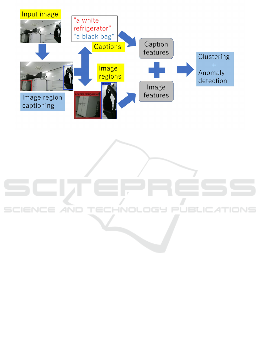
Figure 1: Processing steps of the proposed method.
3.2 Generating Captions of an Image
Region
As we stated previously, we use DenseCap (John-
son et al., 2016) to generate captions for m(i) regions
from image H
i
. For simplicity we adopt K regions
(b
b
b
i1
, . . . , b
b
b
iK
) with the highest confidence scores given
by DenseCap and thus m(i) = K.
We used the model of DenseCap which is trained
with Visual Genome (Krishna et al., 2017) and
available to the public. Visual Genome (Krishna
et al., 2017) comprises 94,000 images and 4,100,000
region-grounded captions. Thus we exploit the data
for our anomaly detection via the deep captioning
model of DenseCap.
3.3 Caption Features based on Word
Embedding
In the next step, we obtain the image region features
from each region based on word embedding. First we
omit stopwords such as articles and prepositions from
the caption c
c
c
it
in the region data b
b
b
it
= (r
r
r
it
, c
c
c
it
). It is
widely known that stopwords have little meaning in
natural language processing. As stopwords we used a
list in nltk library
1
of Python. We denote the remain-
ing word sequence by c
c
c
0
it
.
Then we obtain the distributed representation of
words using Word2Vec. Word2Vec returns respective
vectors U
U
U
it1
, . . . , U
U
U
itT
of the words w
1
, . . . , w
T
, where
T represents the number of words in c
c
c
0
it
. We set the
1
https://www.nltk.org/index.html
number of the dimension of the distributed represen-
tation to 300. We also obtain the normalized coordi-
nates r
r
r
0
it
of the center from the coordinates r
r
r
it
of the
target region with Eqs. (1) and (2). The caption fea-
ture vector F
cap
(b
b
b
it
) of the target region is a concate-
nation of the mean M
M
M
it
of the word distributed rep-
resentation which is normalized with its L2-distance
and dr
r
r
0
it
.
M
M
M
it
=
1
T
T
∑
j=1
U
U
U
it j
(3)
F
cap
(b
b
b
it
) = M
M
M
it
⊕ dr
r
r
0
it
, (4)
where d is a hyper-parameter which controls the in-
fluence of w and h. ⊕ represents the concatenation
operator.
3.4 Combination of the Caption
Features and the Image Features
In addition to the caption features, we also generate
the image features F
im
(b
b
b
it
) and the combined features
F
comb
(b
b
b
it
), which is a concatenation of the two kinds
of features.
F
im
(b
b
b
it
) = V
V
V
it
⊕ dr
r
r
0
it
(5)
F
comb
(b
b
b
it
) = M
M
M
it
⊕V
V
V
it
⊕ dr
r
r
0
it
, (6)
Note that the combined features F
comb
(b
b
b
it
) corre-
spond to our method while the other two kinds of fea-
tures F
cap
(b
b
b
it
) and F
im
(b
b
b
it
) serve as baseline methods
in the experiments.
VISAPP 2020 - 15th International Conference on Computer Vision Theory and Applications
328

3.5 Unsupervised Anomaly Detection
based on Clustering
In the last step, we detect anomalies based on clus-
tering from feature vectors F(b
b
b
it
) of the target image
region obtained in the previous step. As we stated
previously, we use BIRCH (Zhang et al., 1997) due to
its efficiency.
In BIRCH, the feature vector F(b
b
b
it
) is assigned
to the closest leaf node of its CF (Clustering Feature)
tree, which abstracts its observation in the form of a
height-balanced tree. Let the CF vector of this leaf
node be (N
k
, S
S
S
k
, SS
k
). When the radius of the addition
of the CF vector of a new example and the CF vector
of its closest leaf exceeds a user-specified parameter
θ, the new example becomes a new leaf node and its
parent node is reconstructed with a standard proce-
dure for a height-balanced tree (Zhang et al., 1997).
We use the distance between the CF vector of F(b
b
b
it
)
and (N
k
, S
S
S
k
, SS
k
) as the degree of anomaly of F(b
b
b
it
).
The target region is detected as anomalous when the
distance exceeds a user-specified threshold R.
4 EXPERIMENTS
4.1 Datasets
We conducted experiments with two kinds of datasets,
each of which contains a sequence of images ex-
tracted from a video clip and additional images
some of which include anomalous regions. The se-
quence of images, which contain no anomalous re-
gion, are used for training and the additional images
are used for testing. We used only indoor images
in the experiments as our Turtlebot 2 with Kobuki
(https://www.turtlebot.com/) is recommended to op-
erate indoor. The first dataset consists of images taken
by our TurtleBot with Microsoft Kinect for Windows
v2 in a room. It contains 4768 images as the se-
quence sampled every second and additional 358 im-
ages including 15 images containing anomalous re-
gions. The 15 images consist of anomalous actions
such as a person with umbrella in a room and anoma-
lous positions such as books on the floor as shown in
Fig. 2. Note that our interests are directed toward
building human-monitoring robots, which explains
our use of in-house data. Tackling larger benchmark
data with higher variations would require more accu-
rate image captioning.
The second dataset consists of images taken in a
refresh corner with a VCR recorder. It contains about
16800 images as the sequence and additional 715 im-
ages including 31 images containing anomalous re-
gions. The 31 images consist of anomalous actions
such as a person under a table and anomalous posi-
tions such as a bag on the floor.
In applying DenseCap, we set K = 10 as the num-
ber of the detected regions for each image. We in-
spected each test image and annotated anomalous re-
gions for evaluating detection methods. In the in-
spection process, an anomalous region was defined as
either an anomalous object, an anomalous action, or
an anomalous position as we explained in Section 2.
The annotation was based on images only and thus
captions were neglected in the process. Figs. 2 and
3 show examples of images in the first and second
datasets, respectively. The left and middle images in
Fig. 3 represent examples of an anomalous action of
hiding under a table
2
and an anomalous position of a
bag on the floor. As the result, the normal and anoma-
lous examples in the test data of the first dataset are
3545 and 35, respectively. On the other hand, they are
7103 and 47 in the second dataset.
4.2 Design of the Experiments
We conducted five kinds of experiments. The first two
were for performance evaluation: one with all data
and the other for plotting the learning curves. The
next two were for investigating the dependencies on
parameters: one for the threshold parameter θ of the
radius of a leaf node in building the CF tree and the
other for the threshold R of anomaly detection. The
last one was an ablation study of the coordinate infor-
mation dr
r
r
0
it
. The run-time of the employed anomaly
detection methods was negligible compared to the
sampling time of one second. In the first kind of ex-
periments, the detection performance was measured
in terms of precision, recall, F measure, and AUC
(Area under the ROC curve). In the second kind of
experiments, a varying proportion of the training data
were selected randomly, and for each proportion a de-
tection method is applied 10 times to different data.
We report the average performance in AUC.
As baseline methods, we used F
cap
(b
b
b
it
) and
F
im
(b
b
b
it
). To obtain V
V
V
it
, we used VGG-16 (Simonyan
and Zisserman, 2015)
3
. Since our training data is
unlabeled, we used a public model VGG-16 which
was trained with ImageNet (Deng et al., 2009). The
4096-dimensional image features were obtained with
VGG-16 for each region detected with DenseCap and
resized to 224 × 224 pixels. In this sense, the base-
line method with F
im
(b
b
b
it
) also exploits DenseCap for
2
Schools in Japan teach students to take this action un-
der strong shakes during an earthquake.
3
https://keras.io/ja/applications/
Detecting Anomalous Regions from an Image based on Deep Captioning
329
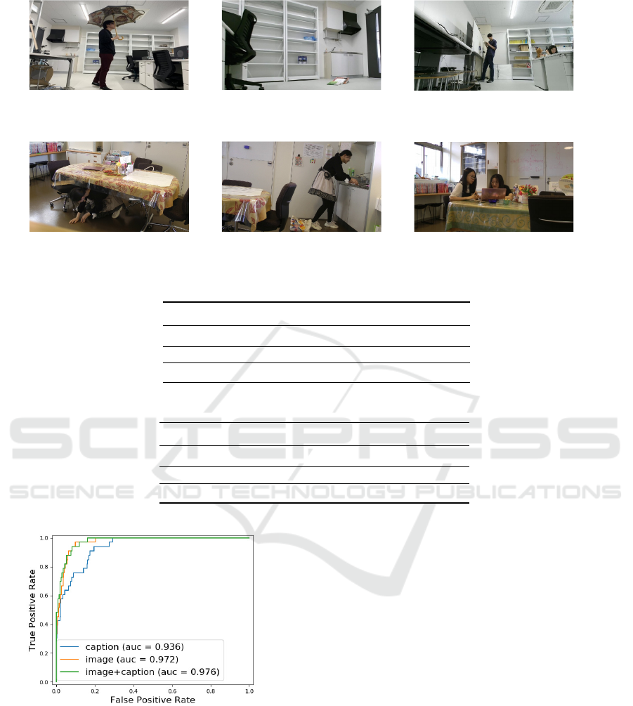
Figure 2: Examples of images in the first dataset. The left and middle images contain anomalous regions (a man with an
umbrella and a book on the floor, respectively) while the right one does not.
Figure 3: Examples of images in the second dataset. The left and middle images contain anomalous regions (a woman under
a table and a bag on the floor, respectively) while the right one does not.
Table 1: Recall, precision, and F measure in the first data.
Precision Recall F measure
Caption 0.500 0.303 0.377
Image 0.464 0.394 0.426
Image + Caption 0.533 0.485 0.508
Table 2: Recall, precision, and F measure in the second data.
Precision Recall F measure
Caption 0.0165 0.0638 0.0262
Image 0.0404 0.0851 0.0548
Image + Caption 0.0654 0.1489 0.0909
Figure 4: ROC curve and AUC in the first data.
detecting salient regions but not the generated cap-
tions. In most of the experiments, we used R = 0.7,
R = 1.0 and R = 1.2 for the caption features F
cap
(b
b
b
it
),
the image features F
im
(b
b
b
it
), and their combinations
F
comb
(b
b
b
it
), respectively, which were determined by
parameter tuning. We are going to investigate the
influence of R in the fourth kind of experiments.
Throughout the experiments, the horizontal and ver-
tical sizes of the images were w = 720 and h = 404.
DenseCap also shrunk the original image size 1920
× 1080 pixels to approximately half, i.e., 720 × 404
pixels.
Except in the third and fifth kinds of experiments,
for the threshold θ to build the CF tree, we used θ =
0.1 for all features. As for the hyper-parameter d, we
set d = 2 except in the fifth kind of experiments.
4.3 Results of the Experiments
4.3.1 Performance Evaluation
Table 1 shows that the combined features outperform
the remaining features in precision, recall, and F mea-
sure. Fig. 4 shows that our method, the combined
features, outperforms the other two kinds of features
in AUC.
The learning curve of our method obtained by the
second kind of experiments for the first dataset is
shown in Fig. 5. Note that we adopted logscale for
the training data proportion throughout investigation.
VISAPP 2020 - 15th International Conference on Computer Vision Theory and Applications
330
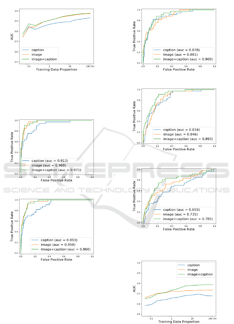
Figure 5: Learning curve of AUC in the first data.
We see that the combined features always outperform
other kinds of features, and the superiority is larger
for smaller samples. We see that our method is still
relatively effective even with 1% of the training data.
Figure 6: ROC curve and AUC in the first data (50%).
Figure 7: ROC curve and AUC in the first data (10%).
Figs. 6-9 show the ROC curves of the three meth-
ods for 50%, 10%, 1%, and 0.1% of the data. We
see that the tendency of the superiority our method is
consistent with that in Fig. 5, and these Figures show
more detailed information.
Table 2 again shows that the combined features
outperforms the remaining two in F measure. Note
that the performance is much lower than in the first
dataset due to the challenging nature of the second
dataset. Figure 10 shows that our combined features
Figure 8: ROC curve and AUC in the first data (1%).
Figure 9: ROC curve and AUC in the first data (0.1%).
Figure 10: ROC curve and AUC in the second data.
outperform the remaining two in AUC.
Figure 11: Learning curve of AUC in the second data.
Detecting Anomalous Regions from an Image based on Deep Captioning
331
Compared with the results of the first dataset, the
performance deteriorated substantially, indicating the
difficulty of this dataset. The learning curve of our
method obtained by the second kind of experiments
for the second dataset is shown in Fig. 11. Though
AUCs are lower than those for the first dataset, we
again see the superiority of the combined features
over the remaining two.
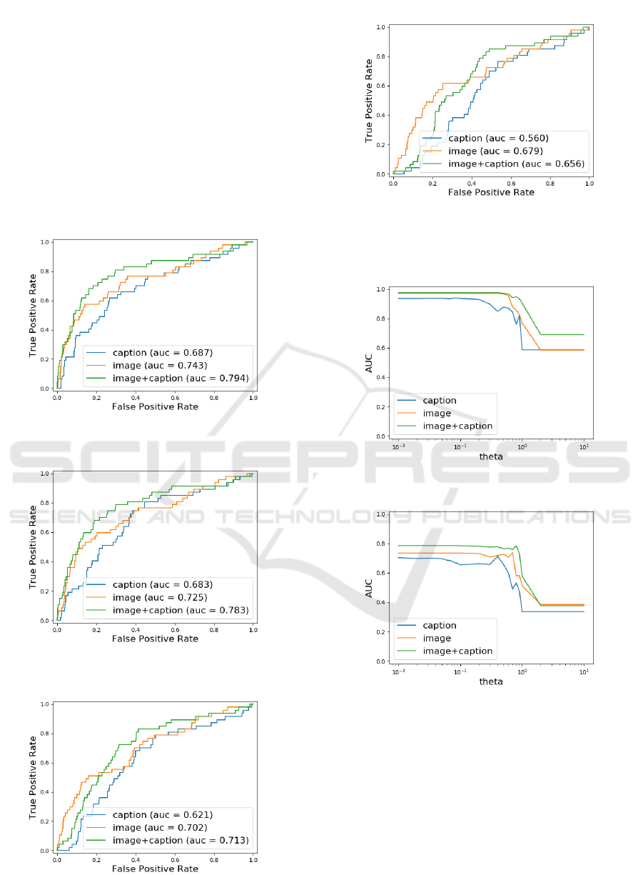
Figs. 12-15 show the ROC curves of the three
methods for 50%, 10%, 1%, and 0.1% of the data.
We again see that the tendency of the superiority our
method is consistent with that in Fig. 11.
Figure 12: ROC curve and AUC in the second data (50%).
Figure 13: ROC curve and AUC in the second data (10%).
Figure 14: ROC curve and AUC in the second data (1%).
Figure 15: ROC curve and AUC in the second data (0.1%).
4.3.2 Parameter Dependencies
Figure 16: Dependency on parameter θ for the first dataset.
Figure 17: Dependency on parameter θ for the second
dataset.
Figure 16 shows the results of the third kind of ex-
periments to investigate the dependency on parameter
θ for the first dataset. The horizontal axis is in log
scale. Figure 16 shows that the performance is stable
in some range but degrades substantially from the end
of the range. We attribute its reason to the fact that
when the value of θ exceeds those of the features all
samples are contained in the same clusters. Figure 17
shows the results for the second dataset. This Figure
shows the same tendency as in Fig. 16, which jus-
tify our analysis above. The combined features have
VISAPP 2020 - 15th International Conference on Computer Vision Theory and Applications
332
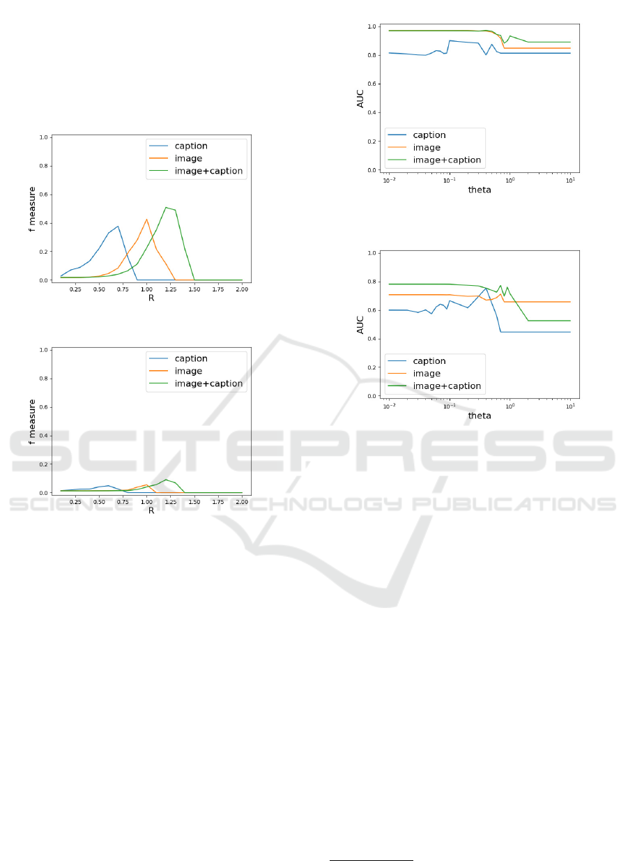
a much wider range of the best values than the base-
line method, which shows that our method is much
less affected by the parameter setting. We again see
the deterioration of the performance compared with
the first dataset, which again indicates the difficulty
of this dataset.
Figure 18: Dependency on parameter R for the first dataset.
Figure 19: Dependency on parameter R for the second
dataset.
For the fourth kind of experiments to investigate
the dependency on the threshold R, we show the re-
sults on the first dataset in Fig. 18. The Figure shows
that the results of the three kinds of features exhibit
different peaks although they are all normalized. One
possible reason is their different dimentionalities: the
image feature has a much higher dimensionality than
the caption feature and thus the pairwise distances are
much larger for the former, which requires larger val-
ues of the threshold for an optimal performance. An-
other possible reason stems from the fact that captions
of two similar images are identical or similar, which
results in smaller pairwise distances and thus the op-
timal values of the threshold are much smaller than
those for the image features. We show the results on
the second dataset in Fig. 19, which show similar ten-
dencies.
Figure 20: Ablation study of the coordinate information (d
= 0) for the first dataset.
Figure 21: Ablation study of the coordinate information (d
= 0) for the second dataset.
4.3.3 Ablation Study and Examples
For the fifth kind of experiments on the influence of
using the coordinate information, we show the results
with the first dataset in Fig. 20. We set d = 0 to ignore
the influence and measured the performance by vary-
ing θ as in the third kind of experiments. Compared
with Fig. 16, the performance of the caption feature
deteriorated while those of the other two features not.
The reason could be attributed to the existence of the
position information in the latter two unlike in the
caption feature. Figure 21 shows the results of the
second dataset, which shows similar tendencies.
To investigate the difference in the caption fea-
tures and the image features, we show in Fig. 22
an example (the purple rectangle) of anomalous re-
gions detected by the caption feature method and
overlooked by the image feature method
4
. To the
region, DenseCap generated a caption “a basket on
the back of the chair”, which helped the caption fea-
tures by providing semantic information not easily
obtained from the image features. Note that even the
caption is wrong in our sense, it was useful in our
4
Our combined feature method successfully detected
this example.
Detecting Anomalous Regions from an Image based on Deep Captioning
333
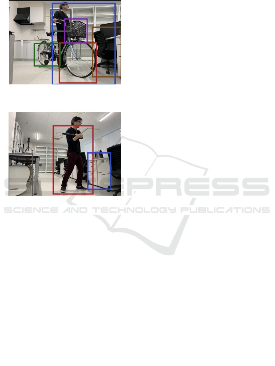
Figure 22: Example of the anomalies detected by the cap-
tion feature method and overlooked by the image feature
method (the purple rectangle).
Figure 23: Example of the anomalies detected by the im-
age feature method and overlooked by the caption feature
method (the red rectangle).
task of detecting anomalous image regions. We also
show in Fig. 23 an example of anomalous regions (the
red rectangle) detected by the method with the image
features and overlooked by the method with the cap-
tion features
5
. To the region, DenseCap generated a
caption “a man playing a game”, which “fooled” the
caption feature method by providing wrong informa-
tion. Though there is no image in which a person is
playing a game in the training data, DenseCap gener-
ated by error a caption “a man playing a video game”
to several regions in training images. The region in
the training data is the cause of the overlook by the
caption feature method.
5 CONCLUSIONS
We proposed an anomalous region detection method
from an image based on deep captioning. Deep cap-
5
Our combined feature method failed to detect this ex-
ample.
tioning allows us to exploit the domain knowledge in
Visual Genome (Krishna et al., 2017), which consists
of a set of pairs of image regions and their captions, in
our task. By processing the captions with a word em-
bedding method Word2Vec, our anomalous detection
is conducted at the semantic level. Our experiments
show the superiority of our method over the baseline
methods which rely on either image features or the
caption features. Recent experiments further showed
that our method is also effective against unseen ob-
jects in the training data and misclassified objects by
image captioning to some extent.
Our ongoing work includes finalizing an au-
tonomous mobile robot for anomaly detection from
its observation. Such a robot is able to integrate vi-
sual information with verbal information and thus has
a large potential in a variety of tasks. The challenge
compared with multi-modal DNNs (Ngiam et al.,
2011) is how to exploit deep captioning model trained
on other data, though our approach can be applied to
domains with much less data. Equipping deep rein-
forcement learning on the robot (Zhu et al., 2017) is
one of our next goals. Integration with our human
monitoring on skeletons (Deguchi and Suzuki, 2015;
Deguchi et al., 2017) and facial expressions (Kondo
et al., 2014; Fujita et al., 2019) are also promising.
Using high-level feedbacks from humans is another
important issue, which would overcome the ineffi-
ciency of online learning with lower-level rewards.
ACKNOWLEDGEMENTS
A part of this work was supported by JSPS KAK-
ENHI Grant Number JP18H03290.
REFERENCES
Arriaga, O., Pl
¨
oger, P. G., and Valdenegro, M. (2017). Im-
age Captioning and Classification of Dangerous Situ-
ations. arXiv preprint arXiv:1711.02578.
Chandola, V., Banerjee, A., and Kumar, V. (2009).
Anomaly Detection: A Survey. ACM Computing Sur-
veys, 41(3).
Deguchi, Y. and Suzuki, E. (2015). Hidden Fatigue Detec-
tion for a Desk Worker Using Clustering of Succes-
sive Tasks. In Ambient Intelligence, volume 9425 of
LNCS, pages 263–238. Springer-Verlag.
Deguchi, Y., Takayama, D., Takano, S., Scuturici, V.-M.,
Petit, J.-M., and Suzuki, E. (2017). Skeleton Clus-
tering by Multi-Robot Monitoring for Fall Risk Dis-
covery. Journal of Intelligent Information Systems,
48(1):75–115.
VISAPP 2020 - 15th International Conference on Computer Vision Theory and Applications
334

Deng, J., Dong, W., Socher, R., Li, L.-J., Li, K., and Li,
F.-F. (2009). ImageNet: A Large-Scale Hierarchical
Image Database. In Proc. CVPR, pages 248–255.
Fujita, H., Matsukawa, T., and Suzuki, E. (2019). Detecting
Outliers with One-Class Selective Transfer Machine.
Knowledge and Information Systems. (accepted for
publication).
Goodfellow, I. J., Pouget-Abadie, J., Mirza, M., Xu, B.,
Warde-Farley, D., Ozair, S., Courville, A. C., and Ben-
gio, Y. (2014). Generative Adversarial Nets. In Proc.
NIPS, pages 2672–2680.
Johnson, J., Karpathy, A., and Fei-Fei, L. (2016). Dense-
Cap: Fully Convolutional Localization Letworks for
Dense Captioning. In Proc. CVPR, pages 4565–4574.
Kato, H., Harada, T., and Kuniyoshi, Y. (2012). Visual
Anomaly Detection from Small Samples for Mobile
Robots. In Proc. IROS, pages 3171–3178.
Kondo, R., Deguchi, Y., and Suzuki, E. (2014). Developing
a Face Monitoring Robot for a Deskworker. In Am-
bient Intelligence, volume 8850 of LNCS, pages 226–
241. Springer-Verlag.
Krishna, R., Zhu, Y., Groth, O., Johnson, J., Hata, K.,
Kravitz, J., Chen, S., Kalantidis, Y., Li, L. J., Shamma,
D. A., Bernstein, M., and Fei-Fei., L. (2017). Vi-
sual Genome: Connecting Language and Vision Us-
ing Crowdsourced Dense Image Annotations. Inter-
national Journal of Computer Vision, 123(1):32–73.
Krizhevsky, A., Sutskever, I., and Hinton, G. E. (2012). Im-
ageNet Classification with Deep Convolutional Neu-
ral Networks. In Proc. NIPS, volume 1, pages 1097–
1105.
Lawson, W., Hiatt, L., and K.Sullivan (2016). Detecting
Anomalous Objects on Mobile Platforms. In Proc.
CVPR Workshop.
Lawson, W., Hiatt, L., and K.Sullivan (2017). Finding
Anomalies with Generative Adversarial Networks for
a Patrolbot. In Proc. CVPR Workshop.
Mahadevan, V., Li, W., Bhalodia, V., and Vasconcelos, N.
(2011). Anomaly Detection in Crowded Scenes. In
Proc. CVPR.
Matsumoto, R., Nakayama, H., Harada, T., and Kuniyoshi,
Y. (2007). Journalist Robot: Robot System Making
News Articles from Real World. In Proc. IROS, pages
1234–1241.
Mikolov, T., Chen, K., Corrado, G., and Dean, J. (2013). Ef-
ficient Estimation of Word Representations in Vector
Space. In Proc. ICLR.
Ngiam, J., Khosla, A., Kim, M., Nam, J., Lee, H., and Ng,
A. Y. (2011). Multimodal Deep Learning. In Proc.
ICML, pages 689–696.
Schlegl, T., Seeb
¨
ock, P., Waldstein, S. M., Schmidt-Erfurth,
U., and Langs, G. (2017). Unsupervised Anomaly
Detection with Generative Adversarial Networks to
Guide Marker Discovery. In Proc. International Con-
ference on Information Processing in Medical Imag-
ing.
Simonyan, K. and Zisserman, A. (2015). Very Deep Convo-
lutional Networks for Large-scale Image Recognition.
In Proc. ICLR.
Suzuki, T., Bessho, F., Harada, T., and Kuniyoshi, Y.
(2011). Visual Anomaly Detection under Temporal
and Spatial Non-Uniformity for News Finding Robot.
In Proc. IROS, pages 1214–1220.
Zhang, T., Ramakrishnan, R., and Livny, M. (1997).
BIRCH: A New Data Clustering Algorithm and its
Applications. Data Min. Knowl. Discov., 1(2):141–
182.
Zhu, Y., Mottaghi, R., Kolve, E., Lim, J. J., Gupta, A., Fei-
Fei, L., and Farhadi, A. (2017). Target-Driven Visual
Navigation in Indoor Scenes Using Deep Reinforce-
ment Learning. In Proc. ICRA, pages 3357–3364.
Detecting Anomalous Regions from an Image based on Deep Captioning
335
