Mediastinal Lymph Node Detection using Deep Learning
Jayant P. Singh
1
, Yuji Iwahori
2
, M. K. Bhuyan
1
, Hiroyasu Usami
2
, Taihei Oshiro
3
and Yasuhiro Shimizu
3
1
Indian Institute of Technology Guwahati, Assam, 781039, India
2
Chubu University, 487-8501, Japan
3
Aichi Cancer Center Hospital, 464-8681, Japan
Keywords:
Convolutional Neural Network, Computed Tomography, Lymph Nodes, U-Net, SVM, ITRST, FCN.
Abstract:
Accurate Lymph Node detection plays a significant role in tumour staging, choice of therapy, and in predict-
ing the outcome of malignant diseases. Clinical examination to detect lymph node metastases alone is tedious
and error-prone due to the low contrast of surrounding structures in Computed Tomography (CT) and to their
varying shapes, poses, sizes, and sparsely distributed locations. (Oda et al., 2017) report 84.2% sensitivity at
9.1 false-positives per volume (FP/vol.) by local intensity structure analysis based on an Intensity Targeted
Radial Structure Tensor (ITRST). In this paper, we first operate a candidate generation stage using U-Net
(modified fully convolutional network for segmentation of biomedical images), towards 100% sensitivity at
the cost of high FP levels to generate volumes of interest (VOI). Thereafter, we present an exhaustive analysis
of approaches using different representations (ways to decompose a 3D VOI) as input to train Convolutional
Neural Network (CNN), 3D CNN (convolutional neural network using 3D convolutions) classifier. We also
evaluate SVMs trained on features extracted by the aforementioned CNN and 3D CNN. The candidate gen-
eration followed by false positive reduction to detect lymph nodes provides an alternative to compute and
memory intensive methods using 3D fully convolutional networks. We validate approaches on a dataset of 90
CT volumes with 388 mediastinal lymph nodes published by (Roth et al., 2014). Our best approach achieves
84% sensitivity at 2.88 FP/vol. in the mediastinum of chest CT volumes.
1 INTRODUCTION
Precise detection and segmentation of enlarged
Lymph Nodes (LNs) play an essential role in the treat-
ment and staging of many diseases, e.g., lung can-
cer, lymphadenopathy, lymphoma, and inflammation
which is essential prior to commencing treatment.
These pathologies can cause affected LN’s to become
enlarged, i.e., swell in size. Nodes are generally con-
sidered to be healthy if they are up to 1 cm in diameter.
Parametric analysis of size, shape and contour, num-
ber of nodes and nodal morphology is critical when
evaluating nodal disease. This assessment is typically
done manually and has potential pitfalls due to the
fact that both normal structures and other patholog-
ical processes can mimic attenuation coefficients of
nodal disease. Furthermore, manual processing is te-
dious and might delay the clinical workflow. This
paper proposes an efficient two-step method to auto-
matically detect enlarged LNs in a patient’s chest CT
scans.
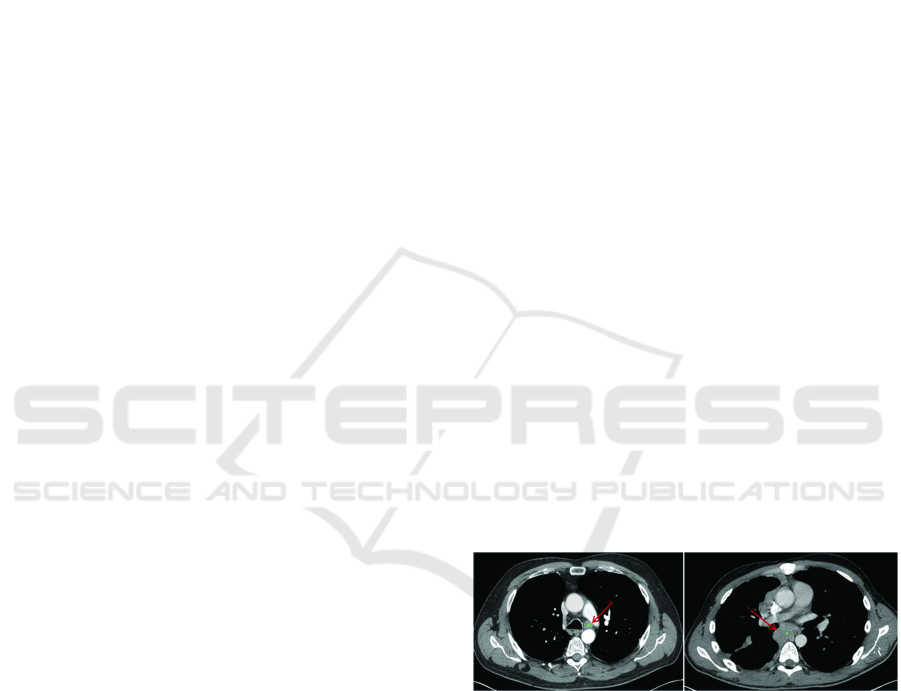
Figure 1: Enlarged Lymph Node (Liu et al., 2016).
2 PREVIOUS WORK
Previous work on computer-aided detection (CADe)
systems for LNs mostly employs direct three-
dimensional information from volumetric CT images.
(Oda et al., 2018) proposed a mediastinal LN detec-
tion and segmentation method from chest CT volumes
based on fully convolutional networks (FCNs), 3D
U-Net. Experimental results showed that 95.5% of
lymph nodes were detected with 16.3 false positives
per CT volume but due to huge number of parame-
ters, the model is likely to overfit and several regions
Singh, J., Iwahori, Y., Bhuyan, M., Usami, H., Oshiro, T. and Shimizu, Y.
Mediastinal Lymph Node Detection using Deep Learning.
DOI: 10.5220/0008948801590166
In Proceedings of the 9th International Conference on Pattern Recognition Applications and Methods (ICPRAM 2020), pages 159-166
ISBN: 978-989-758-397-1; ISSN: 2184-4313
Copyright
c
2022 by SCITEPRESS – Science and Technology Publications, Lda. All rights reserved
159
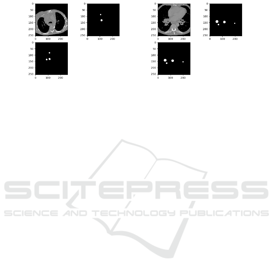
Figure 2: Candidate Generation Results (U-Net): Top Left →Axial Slice; Top Right →Mask; Bottom→Output.
of chest anatomies should be included in dataset in
order to moderate the size imbalance between classes
and prevent oversegmentation. (Barbu et al., 2011)
and (Feulner et al., 2013) performed boosting-based
feature selection and integration over a large num-
ber of 3D Haar-like and steerable features followed
by verification using gradient-aligned features to ob-
tain a strong binary classifier for detecting LNs. Due
to the inherent high dimensionality and a large num-
ber of parameters, modeling complex 3D image struc-
tures for LN detection is non-trivial. Nevertheless,
interpretation of the volumetric context through the
selected model is vital for the accurate detection of
LNs. Particularly, lymph nodes have similar attenu-
ation relative to adjacent anatomic structures such as
vessels, heart, and esophagus. This results in large
number of false-positives (FP), to assure a moder-
ately high detection sensitivity as in (Feuerstein et al.,
2009), (Feuerstein et al., 2012) or only limited sensi-
tivity levels (Barbu et al., 2011) and (Feulner et al.,
2013). The good sensitivities achieved at low FP
range in (Barbu et al., 2011) are not directly com-
parable with the other studies since (Barbu et al.,
2011) report on axillary (83.0% detection rate with
1.0 false positive per volume on 131 volumes con-
taining 371 LN), pelvic and only some parts of the ab-
dominal regions (80.0% detection rate with 3.2 false
positives per volume on 54 volumes containing 569
LN). (Liu et al., 2016) performed simultaneous seg-
mentation of multiple anatomic structures by multi-
atlas label fusion followed by candidate generation by
random forest classification and SVM classification
on chest CT volumes from 70 patients. (Oda et al.,
2017) obtained candidate regions using the Intensity
Targeted Radial Structure Tensor (ITRST) filter and
removed false positives (FPs) using the support vec-
tor machine classifier achieving 84.2% sensitivity at
9.1 FP/vol for mediastinal LN. However, some lymph
nodes initially detected by the ITRST filter are re-
moved by the SVM classifier. We build upon the deep
learning techniques to prevent generating such false
negatives. (Roth et al., 2014) proposed a new 2.5D
representation for LN detection using the deep con-
volutional neural network (CNN) and reported 70%
sensitivity at 3 false positives per volume. However,
(Roth et al., 2014) do not explore the results of deep
learning in candidate generation and 3D convolutions
during false positive reduction. We also provide an
exhaustive analysis of different models with different
input representations, including 2.5D used by (Roth
et al., 2014). Extensions of FCNs to 3D medical data
have been proposed for LN detection, but the com-
putational cost and memory consumption are still too
high to be efficiently implemented in today’s general
computer graphics hardware units.
3 METHODOLOGY
The method can be best described as a unidirectional
pipeline consisting of broadly two sections, 3.1 and
3.2.
Section 3.1 purely focuses on finding the location
of probable enlarged lymph nodes in the mediastinum
of input chest CT volume and hence called Candi-
date Generation. It is deliberately operated at very
high sensitivity so that almost all lymph nodes are de-
tected. However, this also results in a large number of
false positives that need to be eliminated. Section 3.2
purely focuses on the reduction of false positives and
hence called False Positive Reduction.
3.1 Candidate Generation
We refer to the following methods for generation of
LN candidates with their respective use-cases.
3.1.1 U-Net
We use a modified U-Net architecture for detecting
LN candidates from mediastinal CT volumes. The U-
Net is a convolutional network architecture for fast
ICPRAM 2020 - 9th International Conference on Pattern Recognition Applications and Methods
160
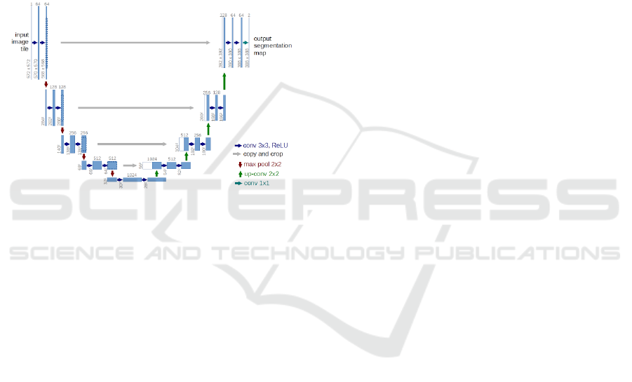
and precise segmentation of biomedical images. As
clearly explained in (Ronneberger et al., 2015), it con-
sists of a contracting path and an expansive path. The
contracting path consists of the repeated application
of two 3 x 3 convolution (same padding), each fol-
lowed by a rectified linear unit and a 2 x 2 max pool-
ing operation for downsampling. At each downsam-
pling, the number of feature channels are doubled. To
avoid overfitting, we use dropout before max pooling
operation that behaves as a regularizer when training
the network. After each convolution layer, we use
batch normalization to reduce covariate shift allowing
each layer to learn by itself a little bit more indepen-
dently of other layers.
Figure 3: U-Net architecture (Ronneberger et al., 2015).
Every step in the expansive path consists of an up-
sampling of the feature map followed by a 3 x 3 up-
convolution (same padding) that halves the number of
the feature channels, a concatenation with the corre-
sponding feature map from the contracting path and
two 3 x 3 convolution each followed by a ReLU. At
the final layer a 1 x 1 convolution is used to map each
16 component feature vector to the desired segmented
image (binary).
3.1.2 Training U-Net
Each CT volume is resampled to a voxel size of 1 mm
x 1mm x 1mm. A window of width 550 HU and level
25 HU is applied to resampled CT volume. All val-
ues less than -250 HU are mapped to -1000 HU, and
those above 300 HU are mapped to 1000 HU. The
network is trained on axial slices of CT volume. (An-
notations in the dataset included only shortest axis
in the axial view of LN in accordance with RECIST
criteria). For a given CT volume, the mask volume
is generated (programmatically) by drawing an ellip-
soid/sphere with center and shortest axis/diameter as
per given annotations. Thereafter, axial slices with at
least one annotated LN are cropped to 256 x 256 pix-
els about the center to contain the mediastinum with
a sufficient margin. Alternatively, the mediastinum
can be extracted by segmenting lungs using a number
of morphological operations followed by appropri-
ate cropping of the region between segmented lungs.
Random rotations, horizontal flips, shear, zoom (0.9-
1.1), horizontal and vertical translations are used for
data augmentation. Both input axial slice and cor-
responding mask are augmented dynamically during
training.
The output image is thresholded at 0.35-0.5, de-
pending on the required sensitivity level (>=0.35
represents part of a detected LN). Subsequently, the
centroids of the detected LNs is found by calculat-
ing moments of contours in the binarized image and
translating coordinates from a cropped 256 x 256 im-
age to original 512 x 512 axial view. The network
is trained till the “test” dice coefficient reaches [0.60,
0.65] range. A much higher dice coefficient may de-
feat the purpose of Section 3.1 to maintain high sen-
sitivity while detecting LNs, which could otherwise
adversely affect Section 3.2 in the aforementioned
pipeline.
3.1.3 Preliminary CADe
For comparison between different models (explained
later) and previous works on mediastinal LN detec-
tion, we use a preliminary CADe system for detecting
LN candidates from mediastinal (Liu et al., 2014) CT
volumes in which lungs are segmented automatically
and shape features by Hessian analysis, local scale,
and circular transformation are computed at voxel-
level. The system uses a spatial prior of anatom-
ical structures (lung, spine, esophagus, heart, etc)
via multi-atlas label fusion before detecting LN can-
didates using a Support Vector Machine (SVM) for
classification.
3.2 False Positive Reduction
Corresponding to each candidate, a 3D VOI of shape
32 x 32 x 32 voxels is extracted with center same
as the candidate centroid. In order to increase train-
ing data variation and to avoid overfitting, each nor-
malized VOI is also flipped (horizontal and vertical),
translated, and rotated along a random vector in 3D
space. Furthermore, each flipped, translated, and ro-
tated VOI is augmented with Gaussian Noise, Gaus-
sian Offset, and Elastic Transform different number
of times depending on the scale of data augmentation.
Different sample and augmentation rates for positive
and negative VOIs are used to obtain a reasonably bal-
anced training set.
When classifying an unseen VOI, we make use of
Test Time Augmentation (TTA). It involves creating
Mediastinal Lymph Node Detection using Deep Learning
161
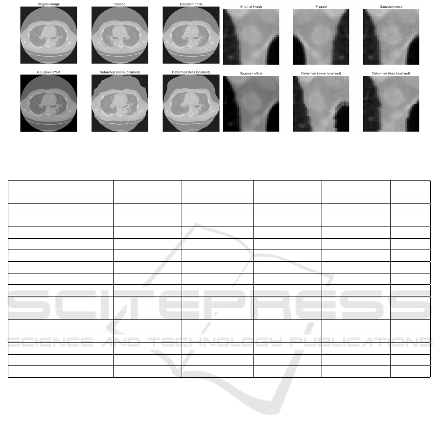
Figure 4: Data Augmentation Types and Positive Axial Lymph Node.
.
Table 1: BS = 32.
BS = 32 PRECISION SENSITIVITY F1 SCORE ROC AUC FP/vol.
2.5D-I (18x) 0.74 (+/- 0.03) 0.82 (+/- 0.06) 0.77 (+/- 0.03) 0.86 (+/- 0.02) 3.08
2.5D-I (34x) 0.79 (+/- 0.04) 0.83 (+/- 0.03) 0.81 (+/- 0.01) 0.87 (+/- 0.01) 3.74
2.5D-II (18x) 0.78 (+/- 0.04) 0.78 (+/- 0.08) 0.78 (+/- 0.03) 0.86 (+/- 0.03) 2.61
2.5D-II (34x) 0.78 (+/- 0.06) 0.82 (+/- 0.06) 0.80 (+/- 0.03) 0.87 (+/- 0.01) 2.97
3D (18x) 0.79 (+/- 0.05) 0.80 (+/- 0.08) 0.80 (+/- 0.05) 0.88 (+/- 0.03) 2.31
3D (34x) 0.80 (+/- 0.04) 0.84 (+/- 0.03) 0.82 (+/- 0.03) 0.89 (+/- 0.03) 2.88
2.5D-I TTA (18x) 0.82 (+/- 0.04) 0.80 (+/- 0.04) 0.81 (+/- 0.01) 0.90 (+/- 0.01) 2.11
2.5D-I TTA (34x) 0.85 (+/- 0.05) 0.83 (+/- 0.05) 0.84 (+/- 0.01) 0.93 (+/- 0.01) 2.78
2.5D-I SVM (18x) 0.79 (+/- 0.04) 0.75 (+/- 0.08) 0.76 (+/- 0.03) 0.87 (+/- 0.02) 2.49
2.5D-I SVM (34x) 0.81 (+/- 0.04) 0.77 (+/- 0.03) 0.79 (+/- 0.01) 0.88 (+/- 0.01) 2.77
2.5D-II SVM (18x) 0.81 (+/- 0.06) 0.74 (+/- 0.10) 0.77 (+/- 0.04) 0.87 (+/- 0.03) 2.37
2.5D-II SVM (34x) 0.82 (+/- 0.06) 0.75 (+/- 0.02) 0.78 (+/- 0.02) 0.88 (+/- 0.03) 2.39
3D SVM (18x) 0.81 (+/- 0.05) 0.76 (+/- 0.09) 0.78 (+/- 0.05) 0.89 (+/- 0.03) 2.20
3D SVM (34x) 0.84 (+/- 0.05) 0.78 (+/- 0.05) 0.81 (+/- 0.03) 0.89 (+/- 0.03) 2.38
2.5D-I TTA SVM (18x) 0.79 (+/- 0.03) 0.75 (+/- 0.02) 0.77 (+/- 0.02) 0.87 (+/- 0.01) 2.24
2.5D-I TTA SVM (34x) 0.83 (+/- 0.03) 0.77 (+/- 0.03) 0.80 (+/- 0.01) 0.89 (+/- 0.01) 2.42
multiple augmented copies of each VOI during test-
ing, having the model make a prediction for each, then
returning an ensemble of those predictions. Augmen-
tations are chosen to give the model the best oppor-
tunity for correctly classifying a given VOI and re-
duce generalization error. Apart from the aforemen-
tioned VOI augmentations, we also use shear angle in
counter-clockwise direction and zoom (0.8-1.2).
Depending on the scale of data augmentation, we
divide the analysis into two broad categories with sub-
categories in each. Let 3x be the number of candi-
date LNs (obtained from Section 3.1), both positive
and negative combined. Following are the broad cat-
egories based on data augmentation scale.
3.2.1 18x
3x increased to 18x using aforementioned data aug-
mentation.
3.2.2 34x
3x increased to 34x using aforementioned data aug-
mentation.
For each broad category following are the sub-
categories:
• 2.5D-I: VOI decomposed into three orthogonal
slices (axial, coronal and sagittal) through the cen-
ter. 32 x 32 x 3 input to CNN;
• 2.5D-II: VOI decomposed into 12 slices (4 axial,
4 coronal and 4 sagittal) through the center. 32 x
32 x 12 input to CNN;
• 3D: VOI as input to 3D CNN (CNN with 3D con-
volutions);
• 2.5D-I TTA: 2.5D-I used with test time augmen-
tation;
ICPRAM 2020 - 9th International Conference on Pattern Recognition Applications and Methods
162

• 2.5D-I SVM: SVM trained on features extracted
by CNN in 2.5D-I;
• 2.5D-II SVM: SVM trained on features extracted
by CNN in 2.5D-II;
• 3D SVM: SVM trained on features extracted by
3D CNN in 3D;
• 2.5D-I TTA SVM: SVM trained on features ex-
tracted by CNN in 2.5D-I TTA;
• Axial: Axial slice through center as input (32 x 32
x 1) to CNN;
• Coronal: Coronal slice through center as input to
CNN;
• Sagittal: Sagittal slice through center as input to
CNN.
3D CNN (Payan and Montana, 2015) uses 3D
convolutions (Figure 5), which apply a 3-dimensional
filter to the input volume, and the filter moves in
three directions to calculate low-level representations.
Their output is a 3-dimensional volume space such as
cube or cuboid. A 2D convolution filter on the other
hand, moves in two directions to give a 2-dimensional
matrix as output. The 3D activation map produced
during the convolution of a 3D CNN is necessary for
analyzing medical data where temporal or volumetric
context is important. The ability to leverage inter-
slice context in a volumetric patch can lead to im-
proved performance but comes with a computational
cost as a result of the increased number of parameters.
4 EVALUATION AND RESULTS
Radiologists labeled a total of 388 mediastinal LNs
as positives in CT images of 90 patients (Roth et al.,
2014). In order to impartially evaluate the perfor-
mance of different approaches mentioned in Section
3.2, close to 100% sensitivity at the LN candidate
generation stage is assumed by feeding the labeled
LNs into the set of CADe LN candidates (Section
3.1.3). The test dice coefficient range [0.60, 0.65] for
candidate generation using U-Net in Section 3.1.2 is
suggested for the same reason. The false-positive de-
tections produced by the CADe system are used as
negative LN candidate examples for training models.
All patients are randomly split into five subsets (at the
patient level) to allow 5-fold cross validation. Note
that the data augmentation (Section 3.2) is performed
at the candidate lymph node level (number of candi-
date lymph nodes per patient can be greater than one)
keeping patient ID information intact to be used later
Figure 5: 3D convolution.
during 5-fold cross validation. Training deep learn-
ing models with RMSprop optimizer on an NVIDIA
GeForce GTX 1060 takes 6 - 22 hrs depending upon
category and sub-category (Section 3.2). We evalu-
ate an approach on the basis of Precision, Sensitivity,
F1 Score, ROC AUC, and False Positives per Volume.
18x and 34x in the table refer to the broad categories
of analysis Section 3.2.1 and Section 3.2.2 respec-
tively, based on the scale of data augmentation. We
perform analysis for batch sizes (BS) 32 and 128 as
summarized in Tables 1 and 2 respectively.
To justify that 3 channels, 1 each of the 3 orthog-
onal views in 2.5D-I; 12 channels, 4 each of the 3
orthogonal views in 2.5D-II and VOI in 3D are not
redundant, we also train CNN model with 1 channel
input under each category of data augmentation con-
taining 1 of the 3 orthogonal views at a time (see Table
3). As expected, in any of the single views, perfor-
mance is not satisfactory with F1 score and ROC in
[0.74, 0.76] and [0.82, 0.86] range, respectively. Sen-
sitivity is comparable with other corresponding sub-
categories but with much larger FP/vol. in [8.48, 9.82]
range.
5 CONCLUSION
Varying a threshold parameter on per-candidate prob-
ability allows us to compute the receiver operating
characteristic (ROC) curves (Figure 6 and Figure 7).
The performance improvement using more data
augmentation (34x) shows that it is beneficial for
CNN to have larger, more varied, and comprehensive
datasets (which is coherent to the computer vision lit-
erature (Krizhevsky et al., 2012), (Zeiler and Fergus,
2014)). 3D CNN seems to perform better than 2D
CNN in 2.5D-I and 2.5D-II because of 3D convo-
lutions exploiting temporal/volumetric information.
2.5D-I with test time augmentation outperforms all
Mediastinal Lymph Node Detection using Deep Learning
163
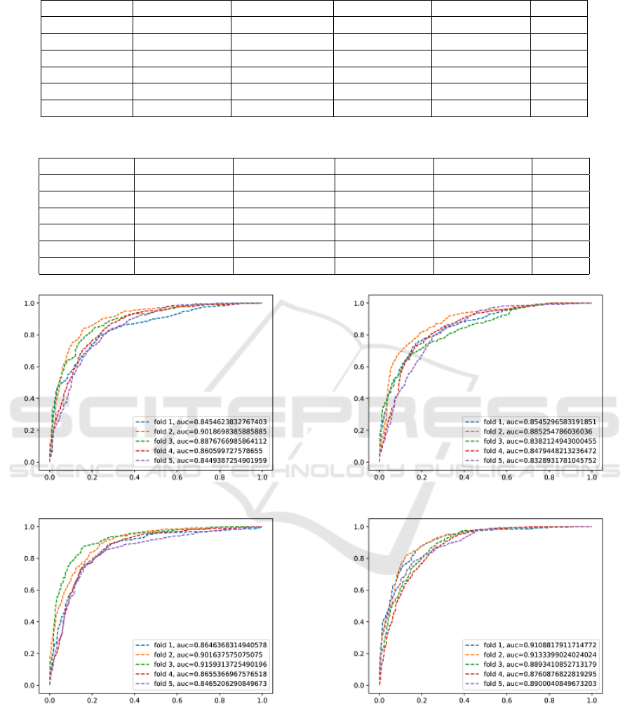
Table 2: BS = 128.
BS = 128 PRECISION SENSITIVITY F1 SCORE ROC AUC FP/vol.
2.5D-I (18x) 0.76 (+/- 0.02) 0.79 (+/- 0.08) 0.77 (+/- 0.03) 0.86 (+/- 0.02) 3.18
2.5D-I (34x) 0.79 (+/- 0.04) 0.81 (+/- 0.04) 0.79 (+/- 0.02) 0.87 (+/- 0.01) 3.51
2.5D-II (18x) 0.78 (+/- 0.05) 0.77 (+/- 0.07) 0.77 (+/- 0.03) 0.86 (+/- 0.02) 2.64
2.5D-II (34x) 0.78 (+/- 0.07) 0.82 (+/- 0.03) 0.80 (+/- 0.03) 0.87 (+/- 0.03) 2.99
3D (18x) 0.78 (+/- 0.04) 0.80 (+/- 0.05) 0.79 (+/- 0.03) 0.87 (+/- 0.03) 2.61
3D (34x) 0.80 (+/- 0.06) 0.83 (+/- 0.04) 0.81 (+/- 0.02) 0.89 (+/- 0.03) 2.73
Table 3: Single Slice.
BS = 32 PRECISION SENSITIVITY F1 SCORE ROC AUC FP/vol.
Axial (18x) 0.67 (+/- 0.04) 0.83 (+/- 0.05) 0.74 (+/- 0.02) 0.84 (+/- 0.02) 9.82
Axial (34x) 0.72 (+/- 0.05) 0.82 (+/- 0.05) 0.76 (+/- 0.02) 0.86 (+/- 0.01) 9.20
Coronal (18x) 0.69 (+/- 0.06) 0.80 (+/- 0.04) 0.74 (+/- 0.03) 0.82 (+/- 0.02) 9.80
Coronal (34x) 0.73 (+/- 0.04) 0.81 (+/- 0.07) 0.76 (+/- 0.02) 0.84 (+/- 0.02) 9.15
Sagittal (18x) 0.72 (+/- 0.06) 0.78 (+/- 0.07) 0.74 (+/- 0.02) 0.83 (+/- 0.02) 8.56
Sagittal (34x) 0.75 (+/- 0.06) 0.78 (+/- 0.07) 0.76 (+/- 0.02) 0.85 (+/- 0.02) 8.48
(a) 2.5D-I (b) 2.5D-II
(c) 3D (d) 2.5D-I TTA
Figure 6: 18x Data Augmentation.
other subcategories with maximum F1 score and AUC
being 0.85 and 0.94, respectively, shown by 2.5D-I
TTA (34x). AUC and ROC exhibit significant im-
provement in sensitivity levels at the range of clini-
cally relevant FP/vol. rates. (Roth et al., 2014) report
70% sensitivity at 3 FP/vol. in the mediastinum (3
fold cross validation on a dataset of 90 patients). (Liu
et al., 2016) report 88% sensitivity at 8 FP/vol. (chest
CT volumes from 70 patients with 316 enlarged me-
diastinal lymph nodes are used for validation), while
our best approach achieves 84% sensitivity at 2.88
FP/vol. in the mediastinum (dataset published by
ICPRAM 2020 - 9th International Conference on Pattern Recognition Applications and Methods
164
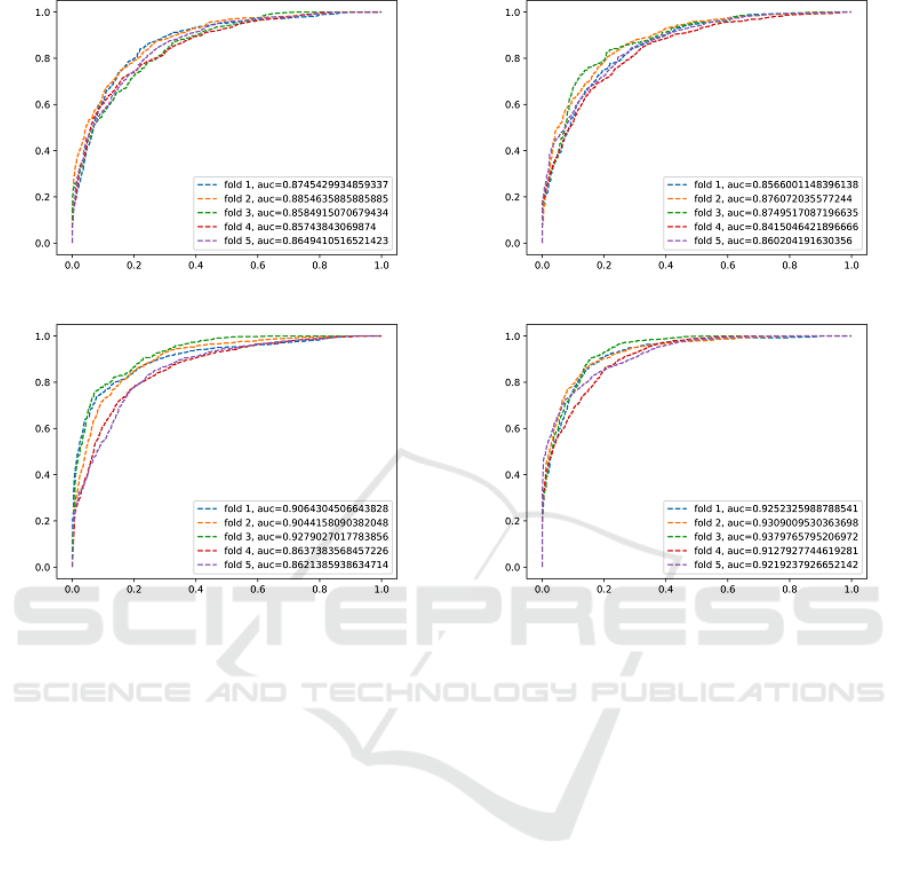
(a) 2.5D-I (b) 2.5D-II
(c) 3D (d) 2.5D-I TTA
Figure 7: 34x Data Augmentation.
(Roth et al., 2014)). Thus, the proposed method of
candidate generation deploying U-Net followed by
false positive reduction using different approaches in-
volving CNN, 3D CNN, SVM (Niu and Suen, 2012),
varying input representations of VOI as explained in
Section 3.2 and results tabulated in Tables 1, 2, 3 can
be used for efficient detection of lymph nodes in a
patient’s chest CT scans. However, if 3D representa-
tions are exploited further for the volumetric context
in serial medical CT data with current advancements
in computing and memory hardware, results can be
greatly improved.
If two or more lymph nodes are very close to each
other then they might be considered as a single lymph
node during candidate generation using U-Net. This
reduces the number of detected lymph nodes which
is undesirable. It remains as future work to improve
the candidate generation step such that it can segment
touching (very close) lymph nodes. To this end, we
propose the use of deep learning architecture aimed
to solve instance segmentation.
ACKNOWLEDGEMENTS
Iwahori’s research is supported by JSPS Grant-in-Aid
for Scientific Research (C) (17K00252) and Chubu
University Grant.
REFERENCES
Barbu, A., Suehling, M., Xu, X., Liu, D., Zhou, S. K.,
and Comaniciu, D. (2011). Automatic detection and
segmentation of lymph nodes from ct data. In IEEE
Transactions on Medical Imaging. IEEE.
Feuerstein, M., Deguchi, D., Kitasaka, T., Iwano, S.,
Imaizumi, K., Hasegawa, Y., Suenaga, Y., and Mori,
K. (2009). Automatic mediastinal lymph node detec-
tion in chest ct. In Medical Imaging 2009: Computer-
Aided Diagnosis. International Society for Optics and
Photonics.
Feuerstein, M., Glocker, B., Kitasaka, T., Nakamura, Y.,
Iwano, S., and Mori, K. (2012). Mediastinal atlas cre-
ation from 3-d chest computed tomography images:
application to automated detection and station map-
ping of lymph nodes. In Medical image analysis. El-
sevier.
Mediastinal Lymph Node Detection using Deep Learning
165

Feulner, J., Zhou, S. K., Hammon, M., Hornegger, J., and
Comaniciu, D. (2013). Lymph node detection and seg-
mentation in chest ct data using discriminative learn-
ing and a spatial prior. In Medical image analysis.
Elsevier.
Krizhevsky, A., Sutskever, I., and Hinton, G. E. (2012). Im-
agenet classification with deep convolutional neural
networks. In Advances in neural information process-
ing systems.
Liu, J., Hoffman, J., Zhao, J., Yao, J., Lu, L., Kim, L., Turk-
bey, E. B., and Summers, R. M. (2016). Mediastinal
lymph node detection and station mapping on chest
ct using spatial priors and random forest. In Medical
physics. Wiley Online Library.
Liu, J., Zhao, J., Hoffman, J., Yao, J., Zhang, W., Turkbey,
E. B., Wang, S., Kim, C., and Summers, R. M. (2014).
Mediastinal lymph node detection on thoracic ct scans
using spatial prior from multi-atlas label fusion. In
Medical Imaging 2014: Computer-Aided Diagnosis.
International Society for Optics and Photonics.
Niu, X.-X. and Suen, C. Y. (2012). A novel hybrid cnn–
svm classifier for recognizing handwritten digits. In
Pattern Recognition. Elsevier.
Oda, H., Bhatia, K. K., Oda, M., Kitasaka, T., Iwano, S.,
Homma, H., Takabatake, H., Mori, M., Natori, H.,
Schnabel, J. A., et al. (2017). Automated mediasti-
nal lymph node detection from ct volumes based on
intensity targeted radial structure tensor analysis. In
Journal of Medical Imaging. International Society for
Optics and Photonics.
Oda, H., Roth, H. R., Bhatia, K. K., Oda, M., Kitasaka, T.,
Iwano, S., Homma, H., Takabatake, H., Mori, M., Na-
tori, H., et al. (2018). Dense volumetric detection and
segmentation of mediastinal lymph nodes in chest ct
images. In Medical Imaging 2018: Computer-Aided
Diagnosis. International Society for Optics and Pho-
tonics.
Payan, A. and Montana, G. (2015). Predicting alzheimer’s
disease: a neuroimaging study with 3d convolutional
neural networks. In arXiv preprint arXiv:1502.02506.
Ronneberger, O., Fischer, P., and Brox, T. (2015). U-net:
Convolutional networks for biomedical image seg-
mentation. In International Conference on Medical
image computing and computer-assisted intervention.
Springer.
Roth, H. R., Lu, L., Seff, A., Cherry, K. M., Hoffman, J.,
Wang, S., Liu, J., Turkbey, E., and Summers, R. M.
(2014). A new 2.5d representation for lymph node de-
tection using random sets of deep convolutional neural
network observations. In International conference on
medical image computing and computer-assisted in-
tervention. Springer International Publishing.
Zeiler, M. D. and Fergus, R. (2014). Visualizing and under-
standing convolutional networks. In European confer-
ence on computer vision. Springer.
ICPRAM 2020 - 9th International Conference on Pattern Recognition Applications and Methods
166
