Parallel Reconstruction of Quad Only Meshes

from Volume Data

Roberto Grosso and Daniel Zint

Visual Computing, Friedrich-Alexander-Universit

at Erlangen-N

urnberg (FAU), Germany

Keywords:

Dual Marching Cubes, Quad Meshing, Parallel Mesh Reconstruction.

Abstract:

We present a method to reconstruct quad only meshes from volume data which mainly consists of two steps:

reconstruction of a quad only mesh and topological simpliﬁcation to reduce the number of irregular vertices.

A novel algorithm is described that computes Dual Marching Cubes (DMC) meshes without using lookup

tables. The meshes are topologically consistent across cell borders, i.e. they are watertight. The output of the

algorithm is a quad only mesh stored in a halfedge data structure. Due to the transitions between voxel layers

in volume data, meshes have numerous quad elements with vertices of valence 3−X −3 −Y, where X, Y ≥5,

and 3 −3 −3 −3. Hence, we simplify the mesh by eliminating these elements wherever possible. Finally, we

brieﬂy describe a CUDA implementation of the algorithms, which allows processing huge amounts of data on

GPU at almost interactive time rates.

1 INTRODUCTION

Iso-surface reconstruction from volume data is a com-

mon processing step in many engineering and scien-

tiﬁc applications, such as surface reconstruction from

range sensor data, analysis and visualization of med-

ical images, or geometry reconstruction of large pro-

tein chains in molecular science. In many cases, vol-

ume data is represented by a hexahedral mesh which

stores a scalar function sampled at the mesh vertices.

In medical applications CT or MRI data are repre-

sented by voxel grids. In this work cell means a voxel

or a hexahedral mesh element. The surface is obtained

by the Marching Cubes (MC) algorithm, which only

requires an iso-value representing the surface as input.

A MC surface shows two major drawbacks. Triangles

are poorly shaped, and the mesh is not topologically

correct, i.e. it might be inconsistent across cell bor-

ders and not homeomorphic to the underlying surface

(Nielson, 2003). The dual marching cubes (DMC) al-

gorithm (Nielson, 2004) generates quad only meshes.

It is based on a lookup table with 23 base cases. A

consistent discretization of the iso-surface across cell

borders requires using the asymptotic decider (Niel-

son and Hamann, 1991; Grosso, 2017) which results

in a large number of special cases, called subconﬁg-

urations in (Nielson, 2003). An alternative strategy

to generate consistent triangulations of the iso-surface

was presented in (Grosso, 2016a; Renbo et al., 2005;

Pasko et al., 1988) and is based on the following ob-

servations. Given an iso-value ι

, the iso-surface is

deﬁned as:

= {(x, y, z) ∈ R

|T (x, y, z) = ι

}, (1)

where T : M → R is the trilinear interpolant deﬁned

on the hexahedral mesh M . The intersection of the

iso-surface with a face of a cell is a set of hyperbolic

arcs. The intersection of the iso-surface with a cell is a

set of closed curves, each being a C

-continuous col-

lection of hyperbolic arcs. Up to four different com-

ponents or branches of the iso-surface can intersect a

cell, resulting in up to four independent closed curves,

hereafter referred to as MC polygons. They are con-

sistent across cell borders if the asymptotic decider is

applied.

DMC computes a vertex representative for each

MC polygon, which should lie on the iso-surface de-

ﬁned by equation (1). In a hexahedral mesh an edge

is shared by four cells. If we connect the vertex repre-

sentatives of the cells sharing a common edge we ob-

tain a quadrilateral. Thus, DMC generates quad only

meshes. If the intersection of the iso-surface with a

cell is computed using the asymptotic decider, it is

guaranteed that the DMC mesh is topologically con-

sistent across cell borders, i.e. it is watertight.

The main contribution of the work is a new DMC

algorithm which does not require a lookup table, gen-

erates watertight meshes, and is simple to parallelize.

102

Grosso, R. and Zint, D.

Parallel Reconstruction of Quad Only Meshes from Volume Data.

DOI: 10.5220/0008948701020112

In Proceedings of the 15th International Joint Conference on Computer Vision, Imaging and Computer Graphics Theory and Applications (VISIGRAPP 2020) - Volume 1: GRAPP, pages

102-112

ISBN: 978-989-758-402-2; ISSN: 2184-4321

The algorithm output is a high quality quad only mesh

which accurately represents the underlying geome-

try as deﬁned by equation (1). Neighborhood and

connectivity information is encoded using a halfedge

data structure. Furthermore, we implemented par-

allel smoothing methods to reduce vertices and ele-

ments with valence pattern 3 −X −3 −Y , X, Y ≥ 5

and 3 −3 −3 −3 which commonly appear in DMC

meshes computed from volume data.

In the following, we ﬁrst present a brief review of

previous work emphasizing the problem of topologi-

cal consistency and parallel reconstruction. In Sec. 3

we present the parallel DMC algorithm, and in Sec. 4

we describe our parallel implementation of two mesh

simpliﬁcation techniques. In Sec. 5 we show the per-

formance of the methods presented, and in Sec. 6 we

give some comments on the results. The source code

is available at GitHub (Grosso, 2016b).

2 RELATED WORK

Research contributions in the area of iso-surface ex-

traction from volume data can be classiﬁed into three

main groups, standard Marching Cubes (MC) and its

extensions to resolve topological correctness and con-

sistency; Dual Marching Cubes which extract quad

meshes dual to the MC polygons; and Dual Contour-

ing, which computes an iso-surface from the dual grid

or the dual of an octree.

Methods for computing iso-surfaces based on the

standard MC have to deal with the problem of in-

consistent meshes across cell borders. Furthermore,

MC methods might generate meshes which are not

homeomorphic to the iso-surface as deﬁned by equa-

tion (1). Methods presented so far are either based on

extended lookup tables, or they ﬁrst compute the in-

tersection of the iso-surface with a cell, resulting in a

MC polygon which is consistently triangulated.

After D

urst (D

urst, 1988) observed that MC does

not consistently triangulate the iso-surface across cell

borders, Nielson and Hamann (Nielson and Hamann,

1991) introduced the asymptotic decider to resolve

ambiguities at the cell faces. Natarajan (Natarajan,

1994) discovered interior ambiguities and introduced

an extended lookup table. Chernyaev (Chernyaev,

1995) modiﬁed the lookup table increasing the num-

ber of cases up to 33 in total, which is commonly

called MC33. Different authors proposed new tech-

niques to improve performance or to solve topological

inconsistencies (Lewiner et al., 2003; Cignoni et al.,

2000; Matveyev, 1999; Montani et al., 1994; Niel-

son, 2003; Custodio et al., 2013; Etiene et al., 2012;

Lopes and Brodlie, 2003). For each ambiguous face,

special subcases have to be considered which results

in a large number of conﬁgurations.

Algorithms were presented which resolve ambi-

guities without using a lookup table. The ﬁrst method

to compute iso-surfaces based on the intersection of

the surface with the cell faces was proposed by Pasko

et al. (Pasko et al., 1988). Renbo et al. (Renbo et al.,

2005) developed a triangulation algorithm which does

not use lookup tables. These methods process un-

ambiguous and ambiguous cells in the same manner,

which is much more computational intensive than the

MC algorithm. Grosso (Grosso, 2016a) developed a

hybrid technique which processes unambiguous cells

with the standard MC. Ambiguous cells are triangu-

lated based on a set of rules applied to the MC poly-

gons. This method has the advantage of not relying

on lookup tables in ambiguous cases.

In order to improve performance and to overcome

the problem of generating a large amount of triangles

many parallel strategies were proposed in literature.

A parallel iso-surface algorithm which is combined

with edge collapses was presented in (Ulrich et al.,

2014; Dupuy et al., 2010). It is a modiﬁcation of the

tandem algorithm introduced in (Attali et al., 2005).

Parallel implementations become more complex if the

output has to be a data structure with connectivity and

neighborhood information. A GPU-based technique

to reconstruct and smooth the iso-surface by repo-

sitioning the vertices without changing mesh topol-

ogy was introduced in (Chen et al., 2015). A method

to compute standard MC on multiple GPUs was de-

scribed in (D’Agostino and Seinstra, 2015). A ma-

jor problem of these algorithms is that they use large

buffers to compute a consistent numbering of the ver-

tex indices. Usually, a unique vertex index is com-

puted by counting cells or edges via a preﬁx sum.

This is not viable in our case, as buffers may be-

come very large. We opted for a different technique

which results in a much simpler algorithm that deliv-

ers good performance results and allows to compute

iso-surfaces from very large volume data.

The Dual Marching Cubes algorithm presented by

Nielson (Nielson, 2004) is a different strategy to re-

construct an iso-surface from a volume data. The in-

tersection of the iso-surface with the cell can be ap-

proximated by a polygon on the cell faces. This is

what we call the MC polygon in the previous section.

The DMC algorithm computes the dual of these MC

polygons. The dual to the MC polygons is a quad only

mesh because each edge in the volume mesh is shared

by four cells. This algorithm relies on the lookup ta-

ble introduced in (Nielson, 2003) which consists of

23 basis cases. Ambiguities are resolved by introduc-

ing sub-conﬁgurations. This method is a generaliza-

Parallel Reconstruction of Quad Only Meshes from Volume Data

103

1111

1010

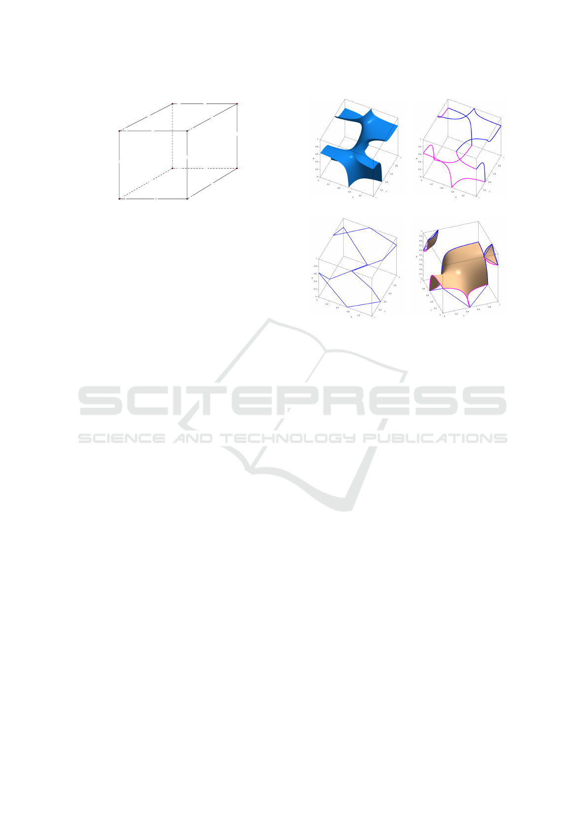
Figure 1: Local index convention for vertices and edges in

a cell.

tion of the SurfaceNets proposed in (de Bruin et al.,

2000; Gibson, 1998). A parallel implementation of

the DMC algorithm is presented in (L

ofﬂer and Schu-

mann, 2012). The method generates a 1-ring neigh-

borhood data structure and approximates the surface

by using error quadrics. Nevertheless, it relies on

large buffers whose size depends on the number of

edges to compute unique vertex indices via preﬁx

sums.

Dual Contouring (DC) (Schaefer and Warren,

2004; Ju et al., 2002) is an alternative method for

extracting iso-surfaces from volume data. It ﬁrst ap-

proximates the data by computing an octree. For each

cell of the octree, the method computes a single ver-

tex representing the surface intersection with the cell.

The vertex is placed within the cell by optimizing

a quadratic functional based on error quadrics. The

method just computes a single vertex for each cell in

the octree, and therefore the resulting mesh might not

be manifold. Subsequently different works were pro-

posed that mainly deal with the problem of comput-

ing manifold meshes out of an octree (Rashid et al.,

2016; Schaefer et al., 2007; Kazhdan et al., 2007;

Zhang et al., 2004). Dual contouring generates tri-

angle meshes from a hierarchical data structure.

3 DUAL MARCHING CUBES

We use the index convention for vertices and edges

shown in Fig. 1. For instance, in the unit reference

cell [0, 1] ×[0, 1] ×[0, 1] we have v

= (0, 0, 0), and

= {v

, v

}. The restriction of the trilinear inter-

polant T to a unit reference cell has the form

F(u, v, w) =

(1 −w)[ f

(1 −u)(1 −v) + f

u(1 −v)

+ f

(1 −u)v + f

uv]

+ w[ f

(1 −u)(1 −v) + f

u(1 −v)

+ f

(1 −u)v + f

uv], (2)

(a) Intersection with cell (b) Hyperbolic arcs on faces

proximating the hyperbolic

arcs

(d) Three MC polygons

Figure 2: MC polygons approximating the intersection of

the iso-surface with the cell faces.

where (u, v, w) ∈ [0, 1]

are local coordinates and f

are the function values at the cell vertices v

. Up

to four branches of the iso-surface obtained from

F(u, v, w) = ι

might intersect the cell. In Fig. 2a

we show an iso-surface with only one component in-

tersecting the cell at all twelve edges. In Fig. 2b

we see the corresponding hyperbolic arcs at the cell

faces, and in Fig. 2c the MC polygon used to approx-

imate the hyperbolic arcs. For each branch of the iso-

surface, DMC selects a single vertex within the cell

which represents the surface. For the case shown in

Fig. 2d three vertices have to be computed.

Each edge in the mesh or voxel grid is shared by

four cells, except for the boundary edges. If a branch

of the iso-surface intersects an edge, it will intersect

all four cells sharing this edge. Therefore, connecting

the representative vertices from each cell will gener-

ate a quadrilateral that is an element of the iso-surface.

If the MC polygons are constructed using the asymp-

totic decider (Nielson and Hamann, 1991), the gener-

ated mesh is topologically consistent across cell bor-

ders. The mesh is called dual, because each vertex in

the MC polygon has a corresponding quadrilateral in

the dual mesh, and each vertex of the dual mesh rep-

resents a MC polygon. The DMC generates meshes

which have less vertices and better shaped elements

than the meshes generated by the standard MC algo-

rithm (Nielson, 2004). Nevertheless, the generated

GRAPP 2020 - 15th International Conference on Computer Graphics Theory and Applications

104

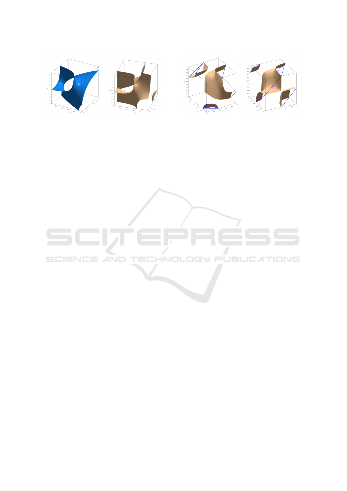
(a) MC case 12 (b) MC case 13

Figure 3: Two conﬁgurations which have the topology of a

cylinder (tunnel) for MC cases 12 and 13.

iso-surface might not be topologically correct. For

certain conﬁgurations which can typically be found

in medical data, the iso-surface (1) will not be home-

omorphic to the reconstructed mesh. The DMC algo-

rithm as it was formulated above cannot reconstruct

tunnels (Grosso, 2016a), Fig. 3. The standard MC

algorithm cannot reconstruct these tunnels either.

The parallel DMC algorithm we propose gener-

ates an indexed face set for the quadrilateral mesh,

where the elements are all consistently oriented. Op-

tionally, a halfedge data structure carrying neighbor

information can be computed. The global structure of

the algorithm we propose consists of three main steps:

1) initialize buffers; 2) compute the DMC mesh; 3)

generate a halfedge data structure. In the initializa-

tion step buffers are created and default values are set

with the help of simple CUDA kernels. In the next

subsections we brieﬂy describe how to compute the

DMC quadrilateral mesh and subsequently generate

the halfedge data structure.

3.1 DMC Quadrilateral Mesh

The DMC quadrilateral mesh is computed with two

CUDA kernels. The ﬁrst kernel proceeds cell wise

and computes the vertex representatives and the

quadrilaterals. The indices constituting a quadrilat-

eral are stored by the kernel in a hash table. We opted

to use a hash table to enable processing of volume

data consisting of hundreds of millions of vertices, see

Sec. 5. The second kernel collects the quadrilaterals

from the hash table into an index buffer. Each thread

started by the ﬁrst kernel has to carry out the follow-

ing processing steps for the cell being processed: 1)

Compute MC polygons, 2) Estimate vertex represen-

tatives for each MC polygon, and 3) Compute and

store quadrilateral indices in a hash table. In order to

improve performance, the kernel returns immediately

if the iso-surface does not intersect the cell.

Figure 4: Two conﬁguration where three branches intersect

the cell, MC case 13.

3.1.1 Computation of MC Polygons

A cell might be intersected by up to four disconnected

branches of the iso-surface. Therefore, we expect

to obtain up to four closed MC polygons. The de-

vice method implemented for this purpose returns the

number of polygons, the size of each of the polygons,

and the indices of the intersected edges. This quan-

tities can be computed in two steps. First, the cell

is processed face wise. The intersection of the iso-

surface with a face is given by a segment, Fig. 2.

For each segment on a face the indices of the start

and end edge are computed. Segments are oriented

such that vertices with function values larger than the

iso-value are located to the left of the segments. Am-

biguous cases are solved with the asymptotic decider

(Nielson and Hamann, 1991). In a second step, seg-

ments are connected to build up closed polygons. The

number of MC polygons, their size, and the indices of

the edges being intersected can be stored in a 64bit

unsigned long integer.

3.1.2 Estimation of Vertex Representatives

Within the cell a vertex that is a representative of the

iso-surface is computed for each surface branch. The

vertex representative must be placed as close as pos-

sible to the iso-surface deﬁned by equation (1). The

different branches intersecting the cell might be very

close to each other, Fig. 4. The estimates for the

vertex representatives must be positioned on the right

surface branch, otherwise the resulting mesh will be

non-manifold, i.e. mesh elements will overlap. We

compute these vertices in two steps. First, an initial

position is estimated. Second, the vertex is moved to-

wards the surface by iteration. The initial position of

the vertex is computed as the mean value (center of

gravity) of the vertices of the MC polygon. This is a

good estimate as can be easily seen from the fact that

branches of the surface within a cell are separated by

asymptotic planes.

Next, the position of the representatives is moved

towards the surface (1) by using the following itera-

Parallel Reconstruction of Quad Only Meshes from Volume Data

105

tion formula:

k+1

= v

+ λ∇F(v

), (3)

where v = (u, v, w) are the local coordinates and λ is

given by

λ = α ·

−F(v

)

||∇F(v

)||

where α is a damping factor. We choose α = 0.25 and

iterate for a maximum of ﬁve steps. Normals are com-

puted at the vertex representative in two steps. First,

the gradient of the scalar function is estimated at the

cell vertices by using central difference. Second, the

gradient is interpolated trilinearly at the position of

the vertex representative and then normalized. We use

central differences because it has a better truncation

error than forward or backward difference. The com-

putation of the gradient using the trilinear interpolant

has the same approximation error as forward differ-

ence, thus producing poor results.

3.1.3 Computation of the Quadrilaterals

Quadrilaterals are computed by connecting vertices of

four neighbor cells sharing a common edge. The edge

must be intersected by the corresponding MC poly-

gons. Quadrilaterals must be consistently oriented. In

contrast to the original MC lookup table (Lorensen

and Cline, 1987), quadrilaterals are oriented such that

their normals point in the same direction as the gradi-

ent of the volume data.

Each quadrilateral is uniquely assigned to an edge

of the volume mesh. Quadrilaterals are stored in a

hash table where the key is the unique index of the

corresponding edge. We use open hashing and lin-

ear probing to ﬁnd an empty bucket in the hash table.

Hash tables were chosen to be twice as large as the

expected number of elements in table. A quadrilat-

eral is represented by an array of four integers. For

each cell, the index of the vertex representative has

to be stored at the right position within this array

to construct quadrilaterals which are consistently ori-

ented. We are using the naming convention presented

in Fig. 1. Fig 5 demonstrates how to save vertex in-

dices properly. Edge e

= {v

, v

} is shared by four

neighbor cells. In the other three cells it will have the

names e

= {v

, v

}, e

= {v

, v

}, and e

= {v

, v

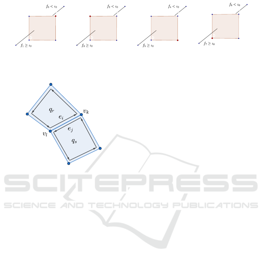
Assume that f

≥ ι

and the index B of the vertex is

stored at the ﬁrst position of the index array. The

thread processing the cell where this edge has the

name e

has to store the index C of the vertex repre-

sentative at the second position in the array. Similarly,

the thread processing the cell where the edge has the

name e

stores the index D at the third position and

ﬁnally, the thread processing the cell where the edge

Table 1: How to build quadrilaterals depending on the edge

conﬁguration. The table indicates the position of the vertex

index in the quadrilateral array.

edge e = {v

, v

} case f

≥ ι

case f

≥ ι

= v

, v

0 0

= v

, v

0 0

= v

, v

3 1

= v

, v

3 1

= v

, v

1 3

= v

, v

1 3

= v

, v

2 2

= v

, v

2 2

= v

, v

0 0

= v

, v

3 1

= v

, v

2 2

= v

, v

2 2

has the name e

stores the vertex A at the fourth po-

sition. All possible cases are summarized in Table 1.

Each quadrilateral is computed by four threads and

stored in a hash table as key, [B, A, D, C].

A kernel is in charge of computing the vertex rep-

resentatives from each cell. The kernel processes the

input data cell wise. For each cell it computes the

vertex representatives and corresponding normals for

each branch of the iso-surface. These vertices are in-

terior to the cell, thus the kernel can assign a unique

global index to the vertices which is required by the

mesh data structure. The index corresponds to the po-

sition of vertex and normal within a buffer and is ob-

tained using atomicAdd on an atomic counter. As in-

dicated above this unique address for vertex and nor-

mal is stored in a hash table, where the key is the

unique index of the edge in the voxel grid being in-

tersected by the corresponding surface branch. The

bucket in the hash table has four entries containing

the indices of the vertices which build a quadrilateral.

The vertices are stored in order to build a consistently

oriented quadrilateral according to the scheme given

in Table 1. The hash table is implemented as an array.

Collisions are solved by using open addressing with

linear probing. We use atomicCAS to test for colli-

sions. At the end the hash table contains all quadrilat-

erals in the mesh.

Finally, a second kernel will collect the quadrilat-

erals from the hash table and save the elements into

an index buffer. Boundaries are easily handled by this

kernel. A bucket in the hash table contains a quadri-

lateral or it is empty. If an entry in a bucket is an

invalid index, the cell was a boundary cell. In this

case no quadrilateral is generated.

GRAPP 2020 - 15th International Conference on Computer Graphics Theory and Applications

106

(a) case e

(b) case e

(d) case e

Figure 5: How to collect vertices from different cells which constitute a quadrilateral.

Figure 6: The distinct threads processing the twin edges

and e

will compute the same key and save them in the

same bucket in the hash table. The neighbor edges will be

connected by the next kernel.

3.2 Halfedge Data Structure

The halfedge data structure is computed using two

kernels. In the ﬁrst kernel, each thread processes

a quadrilateral and collects the local information re-

quired by the data structure. For each vertex we store

the halfedge which starts at the vertex, and for the

face the ﬁrst halfedge is stored. For the four halfedges

in a quadrilateral we store the index of the vertex at

which the halfedge starts, the face and the index of

the next halfedge. This kernel saves the indices of the

halfedges in a hash table. The key is constructed us-

ing the indices of the incident vertices and saved in

a 64bit unsigned long int. The smaller index is

saved in the ﬁrst 32bits, the larger index in the second

32bits. As shown in Fig. 6, distinct threads process-

ing the twin edges e

and e

will compute the same

key based on the indices of the vertices v

, v

and save

them in the same bucket in the hash table. The hald-

edge whose starting vertex has the smaller index is

store at the ﬁrst entry in the bucket, the other at the

second. Global information is collected by a second

kernel which processes the entries of the hash table

and connects twin edges. If a halfedge has no neigh-

bor, it is a boundary edge.

4 MESH SIMPLIFICATION

Due to the transitions between layers in the vol-

ume data, the DMC mesh has numerous quadrilat-

erals with the valence pattern 3 −X −3 −Y , where

X, Y ≥ 5, i.e. two non consecutive vertices with va-

lence 3 and the other two vertices with valence equal

to or larger than 5, Fig. 7a; and quadrilaterals with the

valence pattern 3 −3 −3 −3, Fig. 7b. This elements

can be easily removed from the mesh as follows. For

the case 7a vertices in red are merged into a new ver-

tex and the red element is removed. For the case 7b

edges in red are collapsed moving vertices in red to-

ward vertices in blue. The red elements are removed.

For the conﬁguration 7c no element can be removed

in order to keep the mesh manifold.

4.1 Pattern 3 −X −3 −Y

First note that if two neighbor elements with this va-

lence pattern share a vertex of valence three, the el-

ements can’t be removed from the mesh. Otherwise,

elements with this valence pattern are removed from

the mesh with the following CUDA kernels:

1. Compute vertex valence. For this purpose a ker-

nel iterates through the halfedges and increases

the valence of its vertex by using atomicAdd().

2. Find elements with the valence pattern. For each

quadrilateral a kernel checks the element for the

valence pattern. There is a buffer with an int en-

try for each vertex, a counter, which counts how

often quadrilaterals with this valence pattern share

a vertex with valence three. This way neighbor el-

ements with the same valence pattern that can’t be

removed are identiﬁed easily.

3. Merge vertices with valence three. This kernel

works element wise. For elements with this va-

lence pattern the two vertices with valence three

are merged into a new vertex, Fig. 7a, if the

counter is one for both vertices. Otherwise, a

neighbor element with this valence pattern shares

Parallel Reconstruction of Quad Only Meshes from Volume Data

107

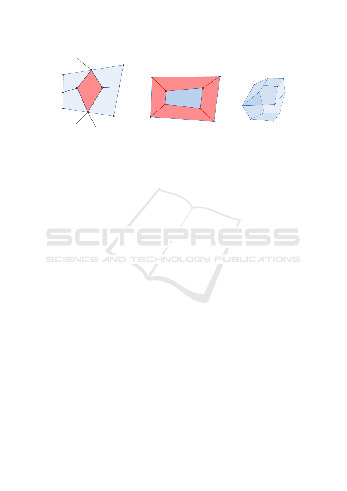
(a) Valence pattern 3 − X − 3 −Y ,

X, Y ≥ 5

(b) Valence pattern 3 −3 −3 −3 (c) This conﬁguration

can’t be removed

Figure 7: Valence pattern 3 −X −3 −Y , where X, Y ≥ 5 and 3 −3 −3 −3. For the case 7a on the left vertices in red are

collapsed into a new vertex, removing the red element. For the case 7b in the middle the edges in red are collapsed moving

the vertices in red toward the vertices in blue. The red elements are removed. For the conﬁguration on the right no element

will be removed in order to keep the mesh manifold.

a vertex of valence three, the element can’t be re-

moved.

4. Remove vertices. This kernel works vertex wise.

It copies vertices to a new vertex buffer, if they

are not marked for removal, and it maps old to

new vertex indices.

5. Remove quadrilaterals. This kernel works ele-

ment wise and copies quadrilaterals to a new el-

ement buffer, if they are not marked for removal.

It uses index mapping from the previous kernel to

connect vertices which form a quadrilateral.

6. Re-build halfedge data structure.

The algorithm requires ﬁve kernels to remove vertices

and elements. Afterwards, the halfedge data structure

has to be re-computed.

4.2 Pattern 3 −3 −3 −3

There are two conﬁgurations for which elements with

this valence pattern can’t be removed from the mesh:

two neighbor elements have the same valence pattern,

e.g. they are the faces of a hexahedron; or the ele-

ments are faces of a conﬁguration as shown in Fig. 7c.

In the latter case, two quadrilaterals sharing the same

four vertices would remain, i.e. the mesh would be

non-manifold. The following processing steps were

implemented to remove elements with the valence

pattern 3 −3 −3 −3:

1. Compute vertex valence. Similar to the kernel

presented in Sec. 4.1.

2. Mark vertices and elements for removal. This ker-

nel processes the mesh element wise. For each el-

ement it tests if all the vertices have valence three.

In this case, the complete neighborhood is recon-

structed. The kernel checks if the element has a

neighbor with the same valence pattern or if it is

the case shown in Fig. 7c. If not, the element

and its four neighbors, Fig. 7b, are marked for

removal.

3. Remove vertices. Similar to the kernel presented

in Sec. 4.1.

4. Remove elements. Similar to the kernel presented

in Sec. 4.1.

5. Re-compute halfedge data structure.

The algorithm requires four kernels to remove ele-

ments from the mesh. We remark that neighborhood

is reconstructed using the halfedge data structure.

5 RESULTS

We evaluate the performance of the parallel DMC and

simpliﬁcation algorithms presented in this work. We

compute the iso-surface from two CT data sets, a hu-

man skull of size 512

×641 shown in Fig. 8 and a

human torso of size 512

×743 for which iso-surfaces

were extracted with different iso-values. For the iso-

value 700, Fig. 9a, we call the data body, and for the

iso-value 1200 skeleton, Fig. 9b. The experiments

were carried out on a desktop computer with an In-

tel Core i7-6700 with 32 GB memory and a NVIDIA

GeForce GTX 1080 8GB. We ﬁrst analyze the perfor-

mance of the parallel DMC algorithm and afterwards

present the effects of mesh simpliﬁcation.

5.1 Parallel DMC

The performance of the parallel DMC is evaluated

by measuring computation time and number of ver-

tices and quadrilaterals generated. We compare the

GRAPP 2020 - 15th International Conference on Computer Graphics Theory and Applications

108

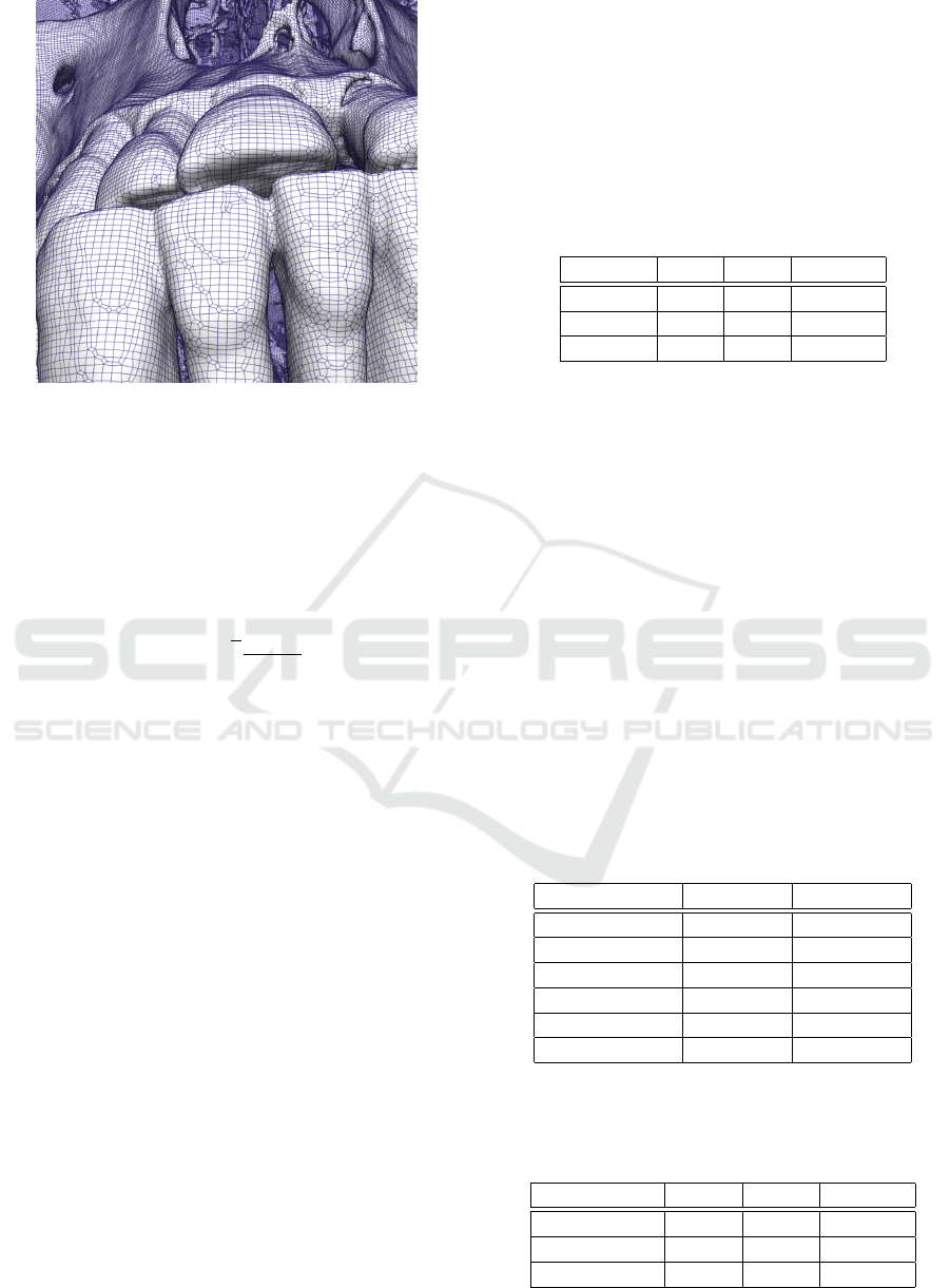
Figure 8: DMC mesh of a CT of a human skull after sim-

pliﬁcation.

results with the corresponding meshes obtained with

the standard MC algorithm. For this purpose we sub-

divide quadrilaterals into triangles. For each element

we select the subdivision which satisﬁes the MaxMin

angle criterion. We also compare the quality of the el-

ements generated by both algorithms. Element qual-

ity is computed using the mean ratio metric,

tri

= 4

√

∑

i=1

, (4)

where A is the signed area of the triangle, and l

the length of their incident edges (Freitag and Knupp,

2002; M. Knupp, 2000).

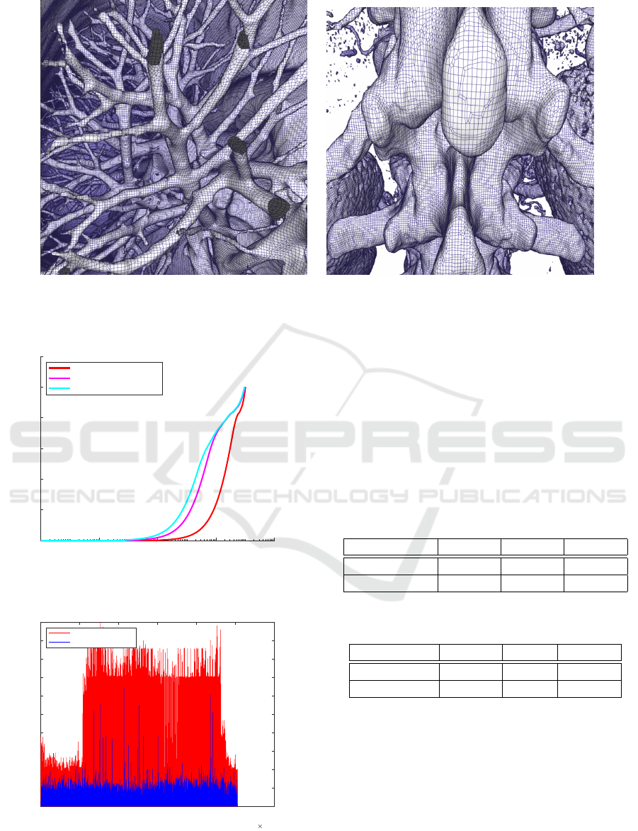
Performance of the DMC in comparison with the

standard MC is given in Table 2. Times are given

in milliseconds. Both algorithms run on the GPU

and for comparison both generate a shared vertex data

structure. Table 3 gives the number of elements gen-

erated by DMC compared to the standard MC algo-

rithm. DMC generates about 1% less vertices and

correspondingly less elements than the standard MC.

The standard MC algorithm is faster than the DMC

algorithm. Nevertheless, it does not generate consis-

tent meshes and the overall quality of the elements is

worse compared to the elements generated by DMC

as shown in Fig. 10. This ﬁgure shows the element

quality for DMC with mesh simpliﬁcation in cyan,

without mesh simpliﬁcation in magenta, and for MC

in red. In this ﬁgure, elements are sorted accord-

ing to their quality. We clearly see that the standard

MC generates a much larger amount of triangles with

a lower quality than the DMC. Mesh simpliﬁcation

slightly increases element quality. For comparison,

quadrilaterals were subdivided into two triangles us-

ing the MaxMin angle criterion. Some quadrilaterals

are thin resulting in triangles which don’t have a good

quality. Element quality and mesh consistency has a

high impact in photo realistic high quality rendering

in graphics applications or mesh processing in com-

putational geometry. This is a main reason why dual

methods for surface reconstruction are preferred over

the standard MC algorithm. Performance was com-

Table 2: Processing time to extract an iso-surface with the

DMC and MC algorithms. The table includes the times re-

quired to generate the halfedge data structure from the DMC

mesh.

skull body skeleton

DMC 85 103 109

MC 54 68 74

halfedge 71 59 87

pared with a C++ implementation of DMC including

a OpenMP parallelization using omp pragmas. The

code has many critical areas due to unique index com-

putations and writing operations. The GPU version is

60 to 77 times faster than the C++ OMP implemen-

tations and around 120 times faster than the sequen-

tial version as shown in Table 4. The back projection

method introduced in Sec. 3.1, equation (3), improves

the accuracy of the DMC mesh, Fig. 11. The plot

in red corresponds to the approximation error without

the projection of the vertex to the surface. The plot in

blue is the error after projection. The approximation

error is measured by comparing the function value at

the vertex with the iso-value normalized to [0, 1]. We

clearly see that the point back projection improves the

accuracy of the vertex representatives.

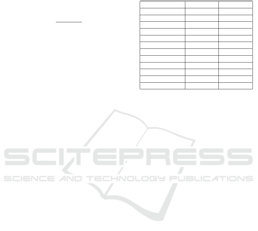
Table 3: Number of elements generated with the DMC and

MC algorithms. The head data set has 512

×641 voxels.

The data set used to generate the the torso and body surfaces

has 512

×743 cells.

vertices elements

skull DMC 5,052,520 5,072,697

skull MC 5,072,707 10,239,432

body DMC 4,249,113 4,234,305

body MC 4,251,835 8,472,218

skeleton DMC 6,294,356 6,278,397

skeleton MC 6,291,993 12,555,936

Table 4: Processing time to extract an iso-surface with the

DMC algorithm on GPU and CPU, including a CPU parallel

implementation with OpenMP. Times are given in millisec-

onds.

skull body skeleton

CUDA 85 103 109

CPU + OMP 6268 5415 8584

CPU 12204 13591 14523

Parallel Reconstruction of Quad Only Meshes from Volume Data

109

(a) DMC mesh showing respiratory tract, iso-value =

700

(b) DMC mesh showing the spine, iso-value = 1200

Figure 9: DMC mesh of a CT of a human torso.

element

0.2

0.4

0.6

0.8

1.2

element quality

DMC

DMC with mesh simplf.

Figure 10: Element quality of DMC in cyan and magenta

compared to MC in red based on the mean ratio metric.

0 1 2 3 4 5 6

vertices

0.1

0.2

0.3

0.4

0.5

0.6

0.7

0.8

0.9

error

without error handling

with error handling

Figure 11: The red plot gives the error of the vertex rep-

resentatives without back projection. The blue plot is the

error after back projection.

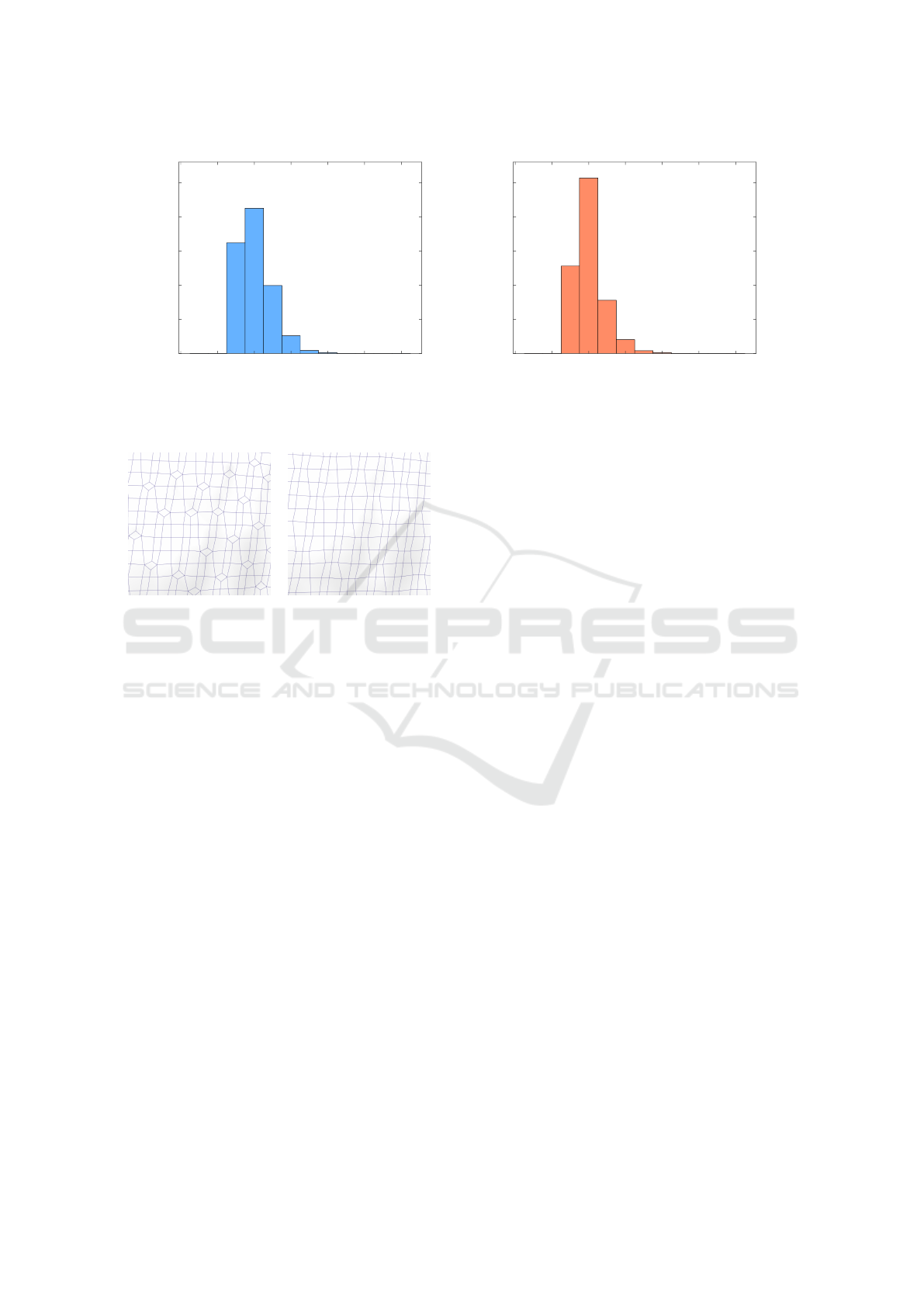
5.2 Mesh Simpliﬁcation

Simpliﬁcation algorithms are evaluated by computa-

tional performance and by the number of elements be-

ing eliminated. The histograms presented in Fig. 12

show that the elimination of elements with valence

patterns 3 −X −3 −Y , X, Y ≥ 5, and 3 −3 −3 −3

considerably reduces the number of irregular vertices.

Table 5: Simpliﬁcation of elements with valence pattern 3 −

X −3 −Y . Times are given in milliseconds.

3 −X −3 −Y skull body skeleton

time 12 9 14

vertices 169,331 161,904 212,795

Table 6: Simpliﬁcation of the valence pattern 3 −3 −3 −3.

Times are given in milliseconds.

3 −3 −3 −3 skull body skeleton

time 7 5 8

vertices 190,292 18,652 165,908

The method implemented to simplify elements

with the valence pattern 3 −X −3 −Y , where X , Y ≥5

eliminates the same number of vertices and elements.

Table 5 gives runtime and total number of elements

removed from the original DMC mesh. For instance,

for the human skull data set it reduces about 3% of

the total number of elements. We remark that the

halfedge data structure has to be recomputed after

mesh simpliﬁcation. Table 6 presents the results ob-

tained with the algorithm for the simpliﬁcation of el-

ements with valence pattern 3 −3 −3 −3. Run times

GRAPP 2020 - 15th International Conference on Computer Graphics Theory and Applications

110

0 2 4 6 8 10 12

valence

0.5

1.5

2.5

vertices

#10

(a) Valence distribution before simpliﬁcation

0 2 4 6 8 10 12

valence

0.5

1.5

2.5

vertices

#10

(b) Valence distribution after simpliﬁcation

Figure 12: Distribution of the vertex valences in the DMC mesh before simpliﬁcation in blue and after in red.

(a) DMC mesh (b) DMC after simpliﬁca-

tion

Figure 13: DMC mesh after removing elements with va-

lence pattern 3 −X −3 −Y and 3 −3 −3 −3

are comparable to the previous case, also eliminat-

ing a similar number of elements, except for the case

of the human torso with iso-value 700, named body

in the table. Due to the geometric properties of the

iso-surface, the body surface does not have many ele-

ments with this valence pattern.

6 CONCLUSIONS

We presented a parallel implementation of the DMC

algorithm which efﬁciently processes volume data

consisting of hundreds of millions of voxels. The

DMC meshes are topologically consistent across cell

borders. This is due to the fact that we compute the

intersection of the iso-surface with the cells using the

asymptotic decider to solve ambiguities. The output

of the algorithm is a quadrilateral mesh stored in a

halfedge data structure. We use the fact that the data

is already on the GPU device and perform some mesh

simpliﬁcation by eliminating vertices and quadrilater-

als with valence pattern 3 −X −3 −Y , X, Y ≥ 5 and

3 −3 −3 −3. This way vertices in the DMC mesh

have better valence distribution. In the implementa-

tion geometric constraints for the simpliﬁcation were

not considered. The DMC algorithm generate meshes

with a better element quality than the standard MC.

REFERENCES

Attali, D., Cohen-Steiner, D., and Edelsbrunner, H. (2005).

Extraction and simpliﬁcation of iso-surfaces in tan-

dem. In Proceedings of the Third Eurographics Sym-

posium on Geometry Processing, SGP ’05, Aire-la-

Ville, Switzerland, Switzerland. Eurographics Asso-

ciation.

Chen, J., Jin, X., and Deng, Z. (2015). Gpu-based polygo-

nization and optimization for implicit surfaces. Vis.

Comput., 31(2):119–130.

Chernyaev, E. V. (1995). Marching cubes 33: Construction

of topologically correct isosurfaces. Technical report.

Cignoni, P., Ganovelli, F., Montani, C., and Scopigno, R.

(2000). Reconstruction of topologically correct and

adaptive trilinear isosurfaces. Computers & Graphics,

24:399–418.

Custodio, L., Etiene, T., Pesco, S., and Silva, C.

(2013). Practical considerations on marching cubes

33 topological correctness. Computers & Graphics,

37(7):840 – 850.

D’Agostino, D. and Seinstra, F. J. (2015). A parallel isosur-

face extraction component for visualization pipelines

executing on gpu clusters. J. Comput. Appl. Math.,

273(C):383–393.

de Bruin, P. W., Vos, F. M., Post, F. H., Frisken-Gibson,

S. F., and Vossepoel, A. M. (2000). Improving tri-

angle mesh quality with surfacenets. In Medical Im-

age Computing and Computer-Assisted Intervention

– MICCAI 2000, pages 804–813, Berlin, Heidelberg.

Springer Berlin Heidelberg.

Dupuy, G., Jobard, B., Guillon, S., Keskes, N., and Ko-

matitsch, D. (2010). Parallel extraction and simpliﬁ-

cation of large isosurfaces using an extended tandem

algorithm. Comput. Aided Des., 42(2):129–138.

Parallel Reconstruction of Quad Only Meshes from Volume Data

111

urst, M. J. (1988). Re: Additional reference to ”marching

cubes”. SIGGRAPH Comput. Graph., 22(5):243–.

Etiene, T., Nonato, L. G., Scheidegger, C., Tienry, J., Pe-

ters, T. J., Pascucci, V., Kirby, R. M., and Silva, C. T.

(2012). Topology veriﬁcation for isosurface extrac-

tion. IEEE Transactions on Visualization and Com-

puter Graphics, 18(6):952–965.

Freitag, L. A. and Knupp, P. M. (2002). Tetrahedral mesh

improvement via optimization of the element condi-

tion number.

Gibson, S. F. F. (1998). Constrained elastic surface nets:

Generating smooth surfaces from binary segmented

data. In Medical Image Computing and Computer-

Assisted Intervention — MICCAI’98, pages 888–898,

Berlin, Heidelberg. Springer Berlin Heidelberg.

Grosso, R. (2016a). Construction of topologically correct

and manifold isosurfaces. Computer Graphics Forum,

35(5):187–196.

Grosso, R. (2016b). tmc. https://github.com/

rogrosso/tmc.

Grosso, R. (2017). An asymptotic decider for robust and

topologically correct triangulation of isosurfaces. In

Proceedings of the Computer Graphics International

Conference, CGI ’17, pages 39:1–39:5, New York,

NY, USA. ACM.

Ju, T., Losasso, F., Schaefer, S., and Warren, J. (2002).

Dual contouring of hermite data. In Proceedings of

the 29th Annual Conference on Computer Graphics

and Interactive Techniques (SIGGRAPH 2002), pages

339–346. ACM Press.

Kazhdan, M., Klein, A., Dalal, K., and Hoppe, H. (2007).

Unconstrained isosurface extraction on arbitrary oc-

trees. In Proceedings of the Fifth Eurographics Sym-

posium on Geometry Processing, pages 125–133.

Lewiner, T., Lopes, H., Vieira, A. W., and Tavares, G.

(2003). Efﬁcient implementation of marching cubes’

cases with topological guarantees. Journal of Graph-

ics Tools, 8(2):1–15.

ofﬂer, F. and Schumann, H. (2012). Generating smooth

high-quality isosurfaces for interactive modeling and

visualization of complex terrains. In VMV.

Lopes, A. and Brodlie, K. (2003). Improving the robust-

ness and accuracy of the marching cubes algorithm

for isosurfacing. IEEE Transactions on Visualization

and Computer Graphics, 9:2003.

Lorensen, W. E. and Cline, H. E. (1987). Marching cubes:

A high resolution 3d surface construction algorithm.

SIGGRAPH Comput. Graph., 21(4):163–169.

M. Knupp, P. (2000). Achieving ﬁnite element mesh qual-

ity via optimization of the jacobian matrix norm and

associated quantities. part i—a framework for sur-

face mesh optimization. Int. J. Numer. Meth. Engng,

48:401–420.

Matveyev, S. V. (1999). Marching cubes: surface complex-

ity measure. In Proceedings of SPIE - The Interna-

tional Society for Optical Engineering, volume 3643,

pages 220–225.

Montani, C., Scateni, R., and Scopigno, R. (1994). A

modiﬁed look-up table for implicit disambiguation of

marching cubes. The Visual Computer, 10(6):353–

355.

Natarajan, B. K. (1994). On generating topologically con-

sistent isosurfaces from uniform samples. The Visual

Computer, 11(1):52–62.

Nielson, G. M. (2003). On marching cubes. IEEE

Transactions on Visualization and Computer Graph-

ics, 9(3):283–297.

Nielson, G. M. (2004). Dual marching cubes. In Proceed-

ings of the Conference on Visualization ’04, VIS ’04,

pages 489–496, Washington, DC, USA. IEEE Com-

puter Society.

Nielson, G. M. and Hamann, B. (1991). The asymptotic de-

cider: Resolving the ambiguity in marching cubes. In

Proceedings of the 2Nd Conference on Visualization

’91, VIS ’91, pages 83–91, Los Alamitos, CA, USA.

IEEE Computer Society Press.

Pasko, A., Pilyugin, V., and Pokrovskiy, V. (1988). Geo-

metric modeling in the analysis of trivariate functions.

Computers & Graphics, 12(3):457 – 465.

Rashid, T., Sultana, S., and Audette, M. A. (2016). Water-

tight and 2-manifold surface meshes using dual con-

touring with tetrahedral decomposition of grid cubes.

Procedia Engineering, 163:136 – 148. 25th Interna-

tional Meshing Roundtable.

Renbo, X., Weijun, L., and Yuechao, W. (2005). A ro-

bust and topological correct marching cube algorithm

without look-up table. In Proceedings of the The Fifth

International Conference on Computer and Informa-

tion Technology, CIT ’05, pages 565–569, Washing-

ton, DC, USA. IEEE Computer Society.

Schaefer, S., Ju, T., and Warren, J. (2007). Manifold dual

contouring. IEEE Transactions on Visualization and

Computer Graphics, 13(3).

Schaefer, S. and Warren, J. (2004). Dual marching cubes:

Primal contouring of dual grids. In Computer Graph-

ics and Applications, 2004. PG 2004. 12th Paciﬁc

Conference on, pages 70–76. IEEE Computer Society.

Ulrich, C., Grund, N., Derzapf, E., Lobachev, O., and

Guthe, M. (2014). Parallel iso-surface extraction and

simpliﬁcation. In WSCG 2014 : Communication

Papers Proceedings, pages 361–368. Vaclav Skala –

Union Agency, Plzen.

Zhang, N., Hong, W., and Kaufman, A. (2004). Dual con-

touring with topology-preserving simpliﬁcation using

enhanced cell representation. In Proceedings of the

Conference on Visualization ’04, pages 505–512.

GRAPP 2020 - 15th International Conference on Computer Graphics Theory and Applications

112