Learning Geometrically Consistent Mesh Corrections
S
,
tefan S
˘
aftescu and Paul Newman
Mobile Robotics Group, Oxford Robotics Institute, University of Oxford, U.K.
{stefan, pnewman}@robots.ox.ac.uk
Keywords:
3D Reconstruction, Depth Refinement, Deep Learning.
Abstract:
Building good 3D maps is a challenging and expensive task, which requires high-quality sensors and careful,
time-consuming scanning. We seek to reduce the cost of building good reconstructions by correcting views of
existing low-quality ones in a post-hoc fashion using learnt priors over surfaces and appearance. We train a
convolutional neural network model to predict the difference in inverse-depth from varying viewpoints of two
meshes – one of low quality that we wish to correct, and one of high-quality that we use as a reference.
In contrast to previous work, we pay attention to the problem of excessive smoothing in corrected meshes. We
address this with a suitable network architecture, and introduce a loss-weighting mechanism that emphasises
edges in the prediction. Furthermore, smooth predictions result in geometrical inconsistencies. To deal with
this issue, we present a loss function which penalises re-projection differences that are not due to occlusions.
Our model reduces gross errors by 45.3%–77.5%, up to five times more than previous work.
1 INTRODUCTION
Dense 3D maps are a crucial component in many sys-
tems and better maps make robots easier to build and
safer to operate. Despite recent progress in hardware
such as the wide availability of GPUs, and algorithms
that scale with the amount of data and the available
hardware, high-quality maps, especially at large scales
and outdoors, remain difficult to build cheaply, often
requiring expensive sensors such as 3D lidars, and
careful, dense scans.
The main motivation of our work is to reduce the
cost of building good dense 3D maps. The reduction
in cost can come from either: a) cheaper but nosier
sensors, such as stereo cameras; b) less data, and there-
fore less time spent densely scanning an area. There
are two ways in which we can produce better recon-
structions with cheaper data. We can learn the kinds of
errors a certain modality produces. For a stereo cam-
era, for example, there will be missing data in areas
without a lot of texture (walls, roads), and the ambi-
guity in depth is usually along the viewing rays. In
addition, we can learn priors for a target environment:
cars usually have known shapes, roads and buildings
do not have holes in them, surfaces tend to be vertical
or horizontal in an urban environment, etc.
We tackle the problem of correcting dense recon-
structions with a convolutional neural network (CNN)
that operates on rasterised views of a 3D mesh as a
post-processing step, following a classical reconstruc-
Mesh Features (View 2)Mesh Features (View 1)
Shared
Weights
abs
Resample from
View 2
Element-wise addition
Element-wise subtraction
Element-wise multiplication
Corrected inverse-depth Corrected inverse-depth
Resampled inverse-depth
Geometric Consistency Error
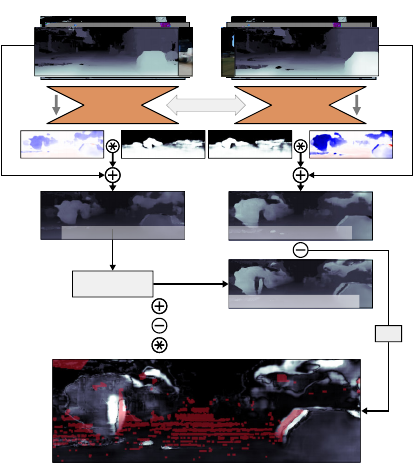
Figure 1: Illustration of geometric consistency for two views
of the same scene a few meters apart. The predictions of our
model can be used to compute corrected depth maps for a
set of views. The corrected depth-maps should be consistent:
they should be describing the same scene. To enforce this,
we densely reproject inverse-depth from View 1 to View 2,
using the corrected depth of View 2. The absolute differ-
ence (bottom) is the inconsistency of View 1 with respect to
View 2. This is minimised during the training of our model,
which enforces geometrically consistent predictions. The
red overlay is the occlusion mask.
tion pipeline. To train this model, we start with two
meshes, a low-quality one and a reference high-quality
one. From each reconstruction, we render multiple
types of images (such as inverse-depth, normals, etc.),
referred to as mesh features, from multiple viewpoints.
We then train the model on the mesh features to pre-
dict the difference in inverse-depth between the high-
quality reconstruction and the low-quality one, thus
enabling us to correct the low-quality mesh.
Previous work (Tanner et al., 2018) has demon-
strated the idea of correcting meshes post-hoc via 2D
rasterised views. We address its two main limitations.
Firstly, we deal with the issue of overly smooth pre-
dictions. We propose changes to the architecture and
training more suitable for our task: we add skip con-
nections from the encoder to the decoder in our
CNN
,
which are known to help in localising edges in pre-
dictions; we propose a loss-weighting method that pe-
nalises incorrect predictions more the closer they are
to an edge. Secondly, predictions on nearby views are
not always consistent, i.e. when applying the predicted
corrections the geometry of the scene is not always
the same. To improve consistency, we employ a view
synthesis based loss, and show that this also improves
the performance of the network. An illustration of the
geometric consistency loss is shown in Figure 1, while
Figure 2 shows an overview of our method.
Our contributions are as follows:
Error correction: We propose a
CNN
model that
is able to correct 2D views of a dense 3D reconstruc-
tion. We propose a novel weighting mechanism to
improve performance around edges in the prediction.
We evaluate it against existing work and show that
we outperform it, especially when images are from
multiple viewpoints.
Geometric consistency: We adapt the photometric
consistency loss that features in related tasks such as
depth-from-mono (Godard et al., 2017) to the task of
correcting reconstructions. This is a novel use of the
loss, which has thus far only been employed on RGB
images. We leverage the existing reconstruction to
compute occlusion masks, and thus exclude from the
loss areas where geometric consistency is impossible.
We show that this use of geometric consistency as an
auxiliary loss further improves our model.
2 RELATED WORK
Several systems for building 3D reconstructions have
been proposed, such as BOR
2
G (Tanner et al., 2015) or
KinectFusion (Newcombe et al., 2011). Our approach
is to correct the output of such a system by looking
at the meshes it builds. As we operate on inverse-
depth images, our work is similar to depth refinement.
Below, we review some of the literature on that topic,
as well as some other methods that our system draws
inspiration from.
Filtering and Optimisation of Depth
Improving depth or disparity images is a well-
researched area, with various methods proposed, some
of which are guided by an additional aligned colour
image. The most straightforward unguided techniques
are based on minimising either on a joint bilateral fil-
ter (
JBF
) (Tomasi and Manduchi, 1998) when filtering,
or Total Generalised Variation (
TGV
) (Bredies et al.,
2010) for optimisation. Guided techniques use another
image aligned with the depth-map to inform the re-
finement. The guide image is used especially around
edges, to modulate the smoothing effect of filtering
or optimisation. For example, Kopf et al. (2007) or
Matsuo et al. (2013) propose variants of a
JBF
for re-
fining depth, while Tanner et al. (2016) demonstrates
a
TGV
-based method that uses both magnitude and di-
rection of colour images to regularise depth maps. An
interesting combination of learning and optimisation
is proposed by Riegler et al. (2016). The Primal-Dual
algorithm (Chambolle and Pock, 2011) normally em-
ployed for
TGV
optimisation is unrolled and included
into a
CNN
model that learns to upsample depth im-
ages. Our work relies on an existing 3D reconstruc-
tion pipeline (Tanner et al., 2015), in which some of
these depth refinement techniques have already been
employed. We focus on post-processing meshes and
fixing errors that cannot easily be fixed in single, live
depth images.
Learnt Depth Refinement and Completion
Some methods for learning depth map refinement and
completion have been recently proposed. Eldesokey
et al. (2018); Uhrig et al. (2017) propose
CNN
model
for solving the KITTI Depth Completion Challenge,
where sparse depth maps produced from laser data
are densified. Hua and Gong (2018) use normalised
convolutions (Knutsson and Westin, 1993) to predict
dense depth maps that have been sparsely sampled.
These methods all rely on having some sort of high-
quality, usually laser, depth information (albeit sparse)
at run-time, and are only designed to fill in the missing
data. In contrast, we only require high-quality data
during training, and our method aims to refine depth
from a low-quality mesh in a more general sense – both
filling in blanks, as well as refining existing surfaces.
A few other methods more closely related in spirit
to ours aim to learn depth refinement using meshes as
reference. Kwon et al. (2015) use dictionary learning
Extracted
mesh features
Stereo Reconstruction
Corrected Reconstruction
3D Fusion (BOR²G)
Geometric
Consistency
Regression
(data, ∇)
Regression
(data, ∇)
Rened
Inverse-depth
Predicted ErrorPredicted Error
Predicted Mask
CNN
CNN
Shared
Weights
Extracted
mesh features
Inverse-depth
labels
Stereo Reconstruction
Lidar Reconstruction
Correction
Training
Rened
Inverse-depth
Predicted ErrorPredicted Error
Predicted Mask
CNN
CNN
Shared
Weights
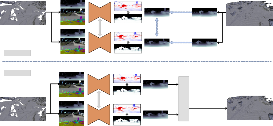
Figure 2: Overview of our method. Our network learns to correct meshes by observing 2D renderings of mesh features and
predicting the error in inverse-depth. In addition to error, our network also predicts a soft mask that is multiplied element-wise
with the error to control which regions of the input inverse-depth image are corrected. During training, inverse-depth images
from a high-quality reconstruction are used to supervise our network, and a geometric consistency loss is applied between
predictions on nearby views, as described in Section 3.2. When using our model to correct meshes, the refined inverse-depth
images of the input mesh are fused into a new 3D reconstruction of higher quality.
to model the statistical relationships between raw RGB-
D images, and high-quality depth data obtained by
fusing multiple depth maps with KinectFusion (New-
combe et al., 2011). Two other recent works use fused
RGB-D reconstruction to obtain high-quality reference
data and train
CNN
s to enhance depth. Zhang and
Funkhouser (2018) uses a colour image to predict nor-
mals and occlusion boundaries, supervised by the 3D
reconstruction, and then formulates an optimisation
problem to fill in holes in an aligned depth image.
Jeon and Lee (2018) introduce a 4000-image dataset
of raw/clean depth image pairs, and train a
CNN
to
enhance raw depth maps. Furthermore, they show
that 3D reconstructions can be obtained with fewer
data and quicker when using their depth-enhancing
network. These methods all rely on live colour images
to guide the refinement or completion of live depth.
That means that only limited data is available for train-
ing. In contrast, our purely mesh-based formulation
allows us to extract many more training pairs from any
viewpoint, removing any viewpoint-specific bias that
might otherwise surface while learning.
Learnt Depth Estimation
Another related line of research has been monocular
depth estimation, which inspires our choices of net-
work architecture and the use of geometry as a source
of self-supervision. Dharmasiri et al. (2019); Godard
et al. (2017); Klodt and Vedaldi (2018); Laina et al.
(2016); Mahjourian et al. (2018); Ummenhofer et al.
(2017); Zhou et al. (2017), etc. propose various
CNN
models for depth estimation from single colour im-
ages. When explicit depth ground-truth is unavailable,
the training is self-supervised using multiview geom-
etry: the predicted depths and relative poses should
maximise the photometric consistency of nearby input
images. In this work, we show how the photometric
consistency loss can be adapted to ensure consistency
between inverse-depth predictions directly, without
need for colour images.
3 METHOD
3.1 Training Data
In contrast to many existing approaches, this work is
about correcting existing reconstructions, and there-
fore we assume the existence of 3D meshes of a scene.
In addition to the low-quality reconstruction we wish
to correct, we also have a high-quality reconstruction
of the same scene. For example, we learn to correct
3D reconstructions from depth-maps using laser recon-
structions as a reference. To build the meshes we train
on, we use the BOR
2
G (Tanner et al., 2015) system.
The training data consists of 2D views of the
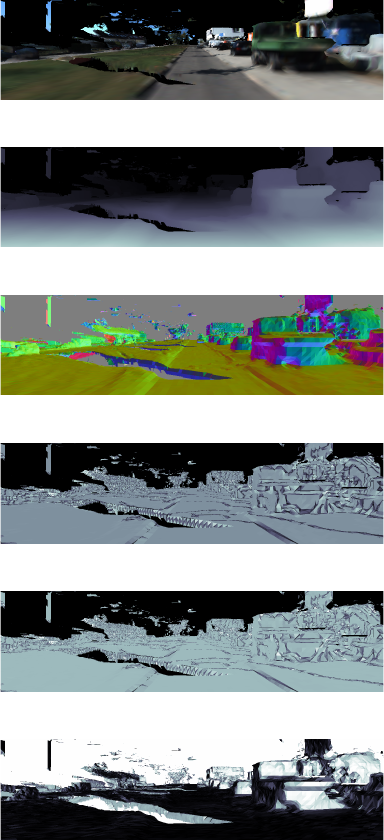
(a) Colour Reconstruction
(b) Inverse-depth
(c) Triangle Surface Normal
(d) Triangle Area
(e) Triangle Edge Length Ratios
(f) Surface to Camera Angle
Figure 3: Example mesh features. We fly a camera through
an existing mesh and at each location produce mesh features.
During training, inverse-depth images of a high-quality mesh
are available, and our model learns a mapping from the mesh
features pictured above to the high-quality inverse-depth.
meshes. We use the same virtual camera to gener-
ate aligned views of the low-quality mesh and the
high-quality mesh for each scene. Because a mesh is
available, we can generate multiple types of images
at each viewpoint. In particular, we generate inverse-
depth, normals, mesh triangle area, mesh triangle edge
ratio (ratio between the shortest and the longest edge
of each triangle), and surface-to-camera angle (Fig-
ure 3). We refer to these images as mesh features. The
ground-truth labels (
∆
) are computed as the difference
in inverse-depth between high-quality and low-quality
reconstructions:
∆(p) = d
hq
(p) − d
lq
(p) (1)
where
p
is a pixel index, and
d
hq
and
d
lq
are inverse-
depth images for the high-quality and low-quality re-
construction, respectively. For notational compactness,
∆(p)
is referred to as
∆
, and future definitions are over
all values of p, unless otherwise mentioned.
Inverse-depth is used instead of depth for several
reasons. Firstly, it emphasises surfaces close to the
camera where more information is available per pixel.
Secondly, background (non-surface) pixels are not pro-
cessed separately – they are assigned a value of zero,
corresponding to points infinitely far away from the
camera. If we used depth, those pixels would either
have to be assigned an arbitrary finite value, which
would result in semantic discontinuities in the output,
or learnt to be ignored by the network, since there is
no standard way to deal with infinite values in a
CNN
.
Finally, another advantage of inverse-depth is that re-
sampling it, which is needed to compute geometric
consistency, is simpler than resampling depth images.
3.2 Geometric Consistency
Intuitively, since the reconstructions we wish to cor-
rect are static, the predictions made from overlapping
views should be geometrically consistent. In other
words, surfaces that appear in a certain location accord-
ing to a prediction should appear in the same location
in all predictions where they are in view.
We resample nearby predicted views according
to the predicted geometry of the current view, and
minimise the absolute difference in inverse-depth. This
dense warping is similar to reprojecting nearby views
into the current view, but has the advantage of being
differentiable, and of generating dense images instead
of sparse reprojected pointclouds. An illustration of
this idea is shown in Figure 1.
Normally, dense warping is used in conjunction
with colour images, where the values of the pixels
are view-independent. Since we are warping inverse-
depth images, where the pixel values depend on the
viewpoint, we need to compute the absolute difference
in the same camera frame.
Concretely, for a view
t
, a nearby view
n
, let
∆
∗
t
be a
CNN
prediction for the target view, let
∆
∗
n
be a
prediction for the nearby view, and let
d
∗
t
= d
lq
t
+ ∆
∗
t
and
d
∗
n
= d
lq
n
+ ∆
∗
n
the corrected inverse-depth images
for the two views. Furthermore, let
p
t
be pixel coor-
dinates in the target view,
K
the intrinsic matrix of
the virtual camera, and
T
n,t
the SE(3) transform from
view
t
to view
n
. We can then define the geometric
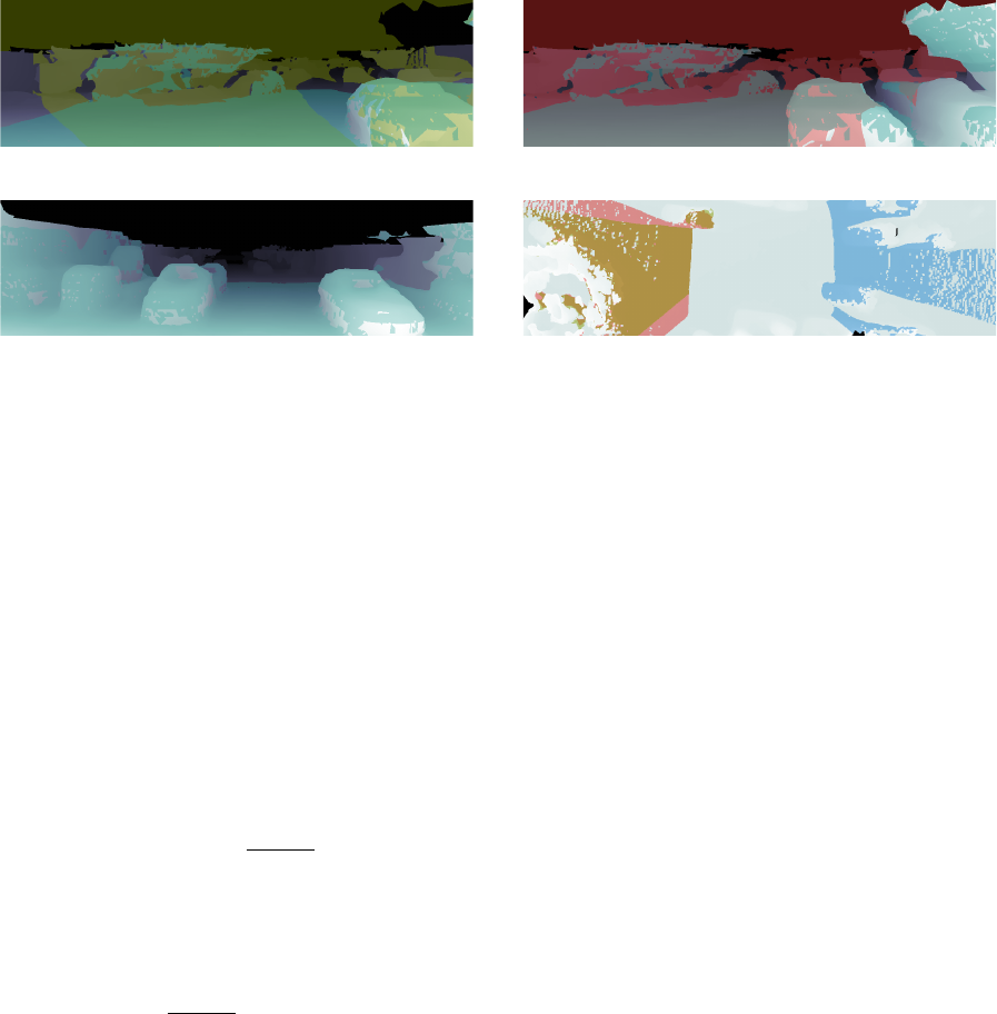
(a) Front-left view. (b) Front-right view.
(c) Back view. (d) Top view.
Figure 4: Visibility masks for views generated at a location. The image regions highlighted in red, green, blue, and cyan
are also visible in the (a) left, (b) right, (c) back, and (d) top views, respectively. (a): inverse-depth view from a dense 3D
reconstruction; the regions visible in the left, and top views are respectively highlighted in green and cyan. (b): a view of the
same scene as (a), 2 m to the right; the regions visible in the left, and top views are respectively highlighted in red and cyan. (c):
a view of the same scene as (a), looking back; the region visible in top view is highlighted in cyan. (d): a view of the same
scene as (a), looking down from 25 m above; the regions visible in the left, right, and back views are respectively highlighted in
red, green, and blue. Areas outside the highlighted regions are occluded – they are not visible from the other view. For example,
distant areas of (a)–(c), such as the sky, are not visible from the top view; the region behind the car on the right in (a) is not
visible from (b). These occluded parts of the image are ignored when computing the geometric consistency loss (Section 3.3.2).
For visualisation purposes, morphological closing has been applied to the visibility masks shown here, to remove some of the
small-scale noise.
inconsistency
d
∗
n,t
−
e
d
∗
n,t
where
d
∗
n,t
is the predicted
inverse-depth from view
t
in the frame of view
n
and
e
d
∗
n,t
is the warped inverse-depth from view n.
They are defined as follows:
e
d
∗
n,t
(p
t
) = d
∗
n
(p
n
), (2)
d
∗
n,t
(p
t
) =
x
(4)
n
x
(3)
n
+ ε
, (3)
where superscripts indicate vector elements,
x
n
is the
3D homogeneous point in view
n
corresponding to
pixel p
t
, and p
n
its projection:
p
n
=
1
x
(3)
n
+ ε
x
(1)
n
x
(2)
n
T
, (4)
x
n
= F
h
x
t
, (5)
x
t
= (p
t
1 d
∗
t
(p
t
))
T
, (6)
F
h
= K
h
T
n,t
K
−1
h
, (7)
K
h
=
K 0
0
T
1
. (8)
The sample pixel
p
n
does not necessarily have in-
teger coordinates, and thus may lie in-between pixels
in the
d
∗
n
grid. Note that we add a small value
ε
with
the same sign as
x
(3)
n
in Equations 3 and 4 to avoid
dividing by zero. Under the mild assumption that sur-
faces between pixels are planar, we can sample
d
∗
n
by
linearly interpolating the four pixels nearest to
p
n
–
another advantage of the inverse-depth formulation.
Occlusion Masks
A common problem with this approach is that views
cannot be consistent in the presence of occlusions. In
our setting, however, since the views are synthetic
(and therefore the intrinsic and extrinsic parameters
are perfectly known), we are able to create occlusion
masks and only apply the geometric consistency loss
where there are no occlusions, as noted in Equation 11.
We compute occlusion masks from the reference
high-quality reconstruction. Each mesh triangle is as-
signed an index by hashing its world frame coordinates.
Then, in addition to mesh features, an image with mesh
triangle indices is generated at each location. For each
pair of views, each pixel of the triangle index image
is resampled from one view into the other in a similar
fashion to the inverse-depth above. Instead of interpo-
lating between the four nearest neighbours, these are
returned as four separate samples. The pixels where
the indices match at least one of the four samples are
considered unoccluded, and the pixels where they do
not are considered occluded (see Figure 4).
Small errors appear due to rasterisation when mesh
triangles are too small, often those that are far away
from the camera. We could avoid these errors by gen-
erating occlusion masks with the OpenGL rasterisation
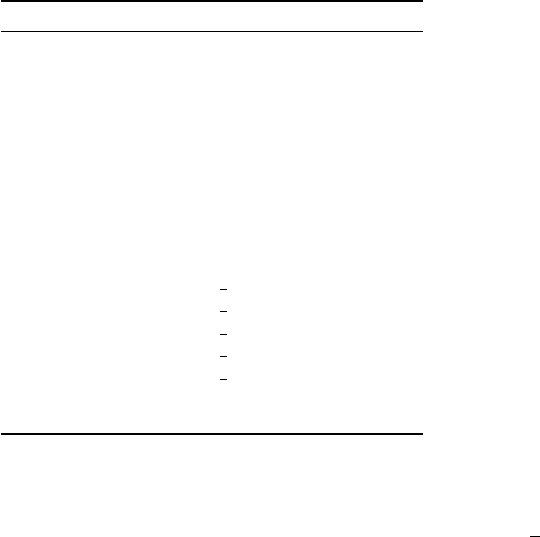
Table 1: Overview of the
CNN
architecture for error predic-
tion.
Block Type Filter Size/Stride Output Size
Input - 96 ×288 × F
Convolution 3 ×3/1 96 ×288 × 64
Residual 3 ×3/1 96 ×288 × 64
Convolution 5 ×5/1 48 ×144 × 64
Max Pool 3 ×3/2 24 × 72 × 64
Residual×2 3 ×3/1 24 × 72 × 64
Projection 3 ×3/2 12 × 36 × 256
Residual×2 3 ×3/1 12 × 36 × 256
Projection 3 ×3/2 6 × 18 × 512
Residual×2 3 ×3/1 6 × 18 × 512
Projection 3 ×3/2 3 × 9 × 1024
Residual×8 3 ×3/2 3 × 9 × 2048
Up-projection 3 ×3/
1
2
6 × 18 ×1024
Up-projection 3 ×3/
1
2
12 × 36 × 512
Up-projection 3 ×3/
1
2
24 × 72 × 256
Up-projection 3 ×3/
1
2
48 ×144 × 128
Up-projection 3 ×3/
1
2
96 ×288 × 32
Residual 3 ×3/1 96 ×288 × 32
Convolution 3 ×3/1 96 ×288 × 2
pipeline when the rest of the data is generated. How-
ever, this greatly increases the space required to store
training data – the number of occlusion masks scales
quadratically with the number of views we want to en-
force consistency between. Generating the occlusion
masks on the fly means that geometric consistency
can be enforced between arbitrary views, so more set-
tings can be explored without regenerating part of the
training data.
3.3 Model
3.3.1 Network Architecture
The model used is an encoder-decoder
CNN
similar to
the one proposed in Tanner et al. (2018). The encoder
is composed of residual blocks based on the ResNet-
50 architecture (He et al., 2016), and the decoder uses
up-convolutions proposed by Shi et al. (2016). U-Net
Ronneberger et al. (2015) style skip connections are
added between the encoder and the decoder to improve
the sharpness of predictions. As a simple way to offer
our model some introspective capabilities, we predict
a soft attention mask (with values
∈ [0, 1]
) in addition
to the error in inverse-depth, as a second output of the
network. This mask is multiplied pixel-wise with the
error prediction to modulate which parts are going to
be used and does not require extra supervision. Table 1
provides an overview for each of the layers of the
proposed CNN.
3.3.2 Loss
The objective function has several components, as fol-
lows. The first term is the data loss that minimises the
error between the output and the label. To compute
this loss, we use berHu norm (Owen, 2007). For large
errors, this behaves in the same way as an
L
2
norm.
For small errors, where the gradients of
L
2
become too
small to drive the error completely to zero,
L
1
norm is
used instead. The advantages of this norm have also
been observed in Laina et al. (2016); Ma and Karaman
(2018). The data loss is defined as follows:
L
data
=
∑
p∈V
W ·
k
∆
∗
− ∆
k
berHu
, (9)
where
p
is the pixel index,
V
is the set of valid pixels
(to account for missing data in the ground-truth),
W
is a per-pixel weight detailed in Section 3.3.3,
∆
∗
and
∆
are the prediction and the target, respectively, and
k · k
berHu
is the berHu norm.
To improve small-scale details and prevent arte-
facts in the prediction, while also allowing for sharp
discontinuities, we also apply a loss on the gradient of
the predictions:
L
∇
=
1
2
∑
p∈V
W·
|
∂
x
∆
∗
− ∂
x
∆
|
+
∂
y
∆
∗
− ∂
y
∆
. (10)
We use the Sobel operator (Sobel and Feldman,
1968) to approximate the gradients in the equation
above.
The geometric consistency loss guides nearby pre-
dictions to have the same 3D geometry, and relies on
reprojected nearby views
e
d
∗
n,t
. For a target view
t
, a set
of nearby views
N
, the set of pixels unoccluded in a
nearby view
U
n
(see Figure 4), this loss is defined as:
L
gc
=
∑
n∈N
∑
p∈U
n
e
d
∗
n,t
− d
∗
n,t
. (11)
Note that
U
n
has no relation to the set of valid pixels
(
V
) from the previous losses, since this loss is only
computed between predictions. This enables the net-
work to make sensible predictions even in parts of the
image which have no valid label.
Finally, we also include an
L
2
weight regulariser,
L
reg
, to reduce overfitting by keeping the weights
small. The overall objective is thus defined as:
L = λ
data
L
data
s
+ λ
∇
L
∇
+ λ
gc
L
gc
+ λ
reg
L
reg
, (12)
where
s
is the scale, and the
λ
s are weights for each
of the components (see Table 2 for values).
3.3.3 Loss Weight
Inspired by the work of Ronneberger et al. (2015) on
U-Nets, we use a loss-weighting mechanism based on
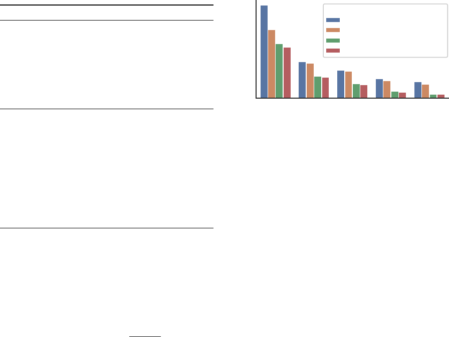
Table 2: Summary of Hyperparameters Used in System.
Symbol Value Description
λ
data
1 Weight of the data loss.
λ
∇
0.1 Weight of the smoothness loss.
λ
gc
0.1
Weight of the geometric consis-
tency loss.
λ
reg
10
−6
Weight of the
L
2
variable regu-
lariser.
w
min
0.1 Minimum per-pixel loss scaling.
w
max
5 Maximum per-pixel loss scaling.
η
max
10
−4
Initial learning rate.
η
min
5 ·10
−6
Final learning rate.
T
max
1.2 ·10
5
Learning rate decay steps.
β
1
0.9
Adam exponential decay rate for
first moment estimates.
β
2
0.999
Adam exponential decay rate for
second moment estimates.
80
Norm at witch gradients are
clipped during training.
16 Batch size.
5 ·10
5
Number of training steps.
the Euclidean Distance Transform (Felzenszwalb and
Huttenlocher, 2012) to emphasise edge pixels when
regressing to the error in depth. We first extract Canny
edges (Canny, 1986) from the ground-truth labels.
Based on these edges, we then compute the per-pixel
weights as:
d(p) = ln(1 + EDT(p))
W(p) = (w
max
− w
min
)
1 −
d(p)
max
p
d(p)
+ w
min
,
(13)
where
W(p)
is the loss weight for pixel
p
,
EDT(p)
is
the Euclidean Distance Transform at pixel
p
, and
w
min
and
w
max
are the desired range of the per-pixel weight.
This will assign
w
max
weight to edge pixels, and lower
weights the farther pixels are from an edge, down to
w
min
for the farthest pixels.
4 EXPERIMENTS
4.1 Experimantal Setup
Training and Inference
The network is implemented in Python using Tensor-
Flow v1.12. Each model is trained on an Nvidia Ti-
tan V GPU. The weights are optimised for 500 000
steps with a batch size of 16 using the Adam opti-
miser (Kingma and Ba, 2015). The learning rate (
η
t
)
is decayed linearly for the first 120 000 steps. Gener-
ating the mesh features takes an average of 52 ms per
view using OpenGL on an Nvidia GTX Titan Black,
# gross error pixels
1.05 1.15 1.25 1.25
2
1.25
3
Threshold
0
1
2
3
4
10
8
Ours (full)
Ours w/o geometric consistency
Uncorrected
Baseline (Tanner et al., 2018)
Model
Figure 5: Gross error correction. For each threshold (Equa-
tion 14), we count how many pixels are incorrect in the
predictions over the test set. Our full model removes 45.3%
of the smaller errors and 77.5% of the gross errors. The
baseline model is unable to effectively handle the multi-view
setup, and fails to correct gross errors.
and inference takes an average of 12.5 ms on the Ti-
tan V. All the training hyper-parameters are defined in
Table 2. The optimiser parameters are the ones sug-
ested by Kingma and Ba (2015), while the rest have
been chosen after a small search to improve validation
metrics.
Dataset
Three sequences from the KITTI visual odometry
(
KITTI-VO
) dataset were used as the input to the re-
construction pipeline. For each sequence, two recon-
structions are built: one from the stereo camera depth-
maps, and one from the laser data. Both the meshes
are generated with a fixed voxel width of 0.2 m. In
the experiments, we show how to learn a correction
of the depth-map reconstruction using the laser recon-
struction as reference. Using OpenGL Shading Lan-
guage (
GLSL
), we create a virtual camera and project
each dense reconstruction into mesh features. We
sample locations along the original trajectory in each
sequence every 0.3m, and at each location we gener-
ate mesh features from four different viewpoints. An
illustration of the viewpoints is shown in Figure 4. For
all experiments, the
KITTI-VO
sequences 00, 05, and
06 are used, from which a total of 96 728 training ex-
amples of size
96 × 288
are generated. We split each
of the mesh feature sequences into three distinct parts:
the first 80% we use as training data, the next 10%
we use for validating hyperparameter choices, and the
last 10% we use for evaluation. All three sequences
are predominantly in urban environments with small
amounts of visible vegetation.
Performance Metrics
We use some metrics common in literature for assess-
ing inverse-depth predictions.

Table 3: Generalisation Capability of Depth Error Correction.
Model Train Test iMAE iRMSE δ < 1.05 δ < 1.15 δ < 1.25
1
δ < 1.25
2
δ < 1.25
3
Uncorrected – 00 1.76 ·10
−2
8.10 · 10
−2
52.71% 79.00% 84.02% 88.73% 90.71%
– 05 1.57 · 10
−2
8.15 · 10
−2
55.11% 80.61% 84.27% 88.30% 90.46%
– 06 2.81 · 10
−2
1.24 · 10
−1
49.47% 72.71% 75.07% 78.64% 80.49%
Ours 05; 06 00 1.45 ·10
−2
8.03 · 10
−2
66.14% 85.27% 89.93% 94.76% 96.82%
00; 06 05 1.19 ·10
−2
7.67 · 10
−2
70.38% 86.31% 90.25% 94.86% 96.99%
00; 05 06 2.37 ·10
−2
1.15 · 10
−1
62.27% 78.14% 81.72% 85.85% 88.20%
Table 4: Depth Error Correction Ablation Study Results.
Model iMAE iRMSE δ < 1.05 δ < 1.15 δ < 1.25 δ < 1.25
2
δ < 1.25
3
Uncorrected 1.85 · 10
−2
8.73 ·10
−2
50.90% 80.77% 85.38% 89.72% 91.35%
Baseline 1.47 · 10
−2
6.25 ·10
−2
63.92% 81.65% 85.90% 90.72% 92.69%
w/ our losses; no GC 1.28 · 10
−2
6.26 ·10
−2
67.77% 84.35% 89.05% 94.16% 96.17%
w/ our losses; GC 1.17 ·10
−2
5.44 ·10
−2
68.66% 84.64% 89.45% 94.81% 96.65%
Ours (no attn; no GC) 1.12 · 10
−2
5.49 ·10
−2
70.47% 87.68% 92.08% 96.35% 97.72%
Ours (no GC) 1.12 · 10
−2
5.63 ·10
−2
71.31% 88.34% 92.41% 96.41% 97.81%
Ours (no attn) 1.02 · 10
−2
5.31 ·10
−2
72.93% 89.27% 93.20% 96.87% 98.10%
Ours (full) 1.06 · 10
−2
5.37 · 10
−2
73.16% 88.94% 92.91% 96.76% 98.05%
Our first metric measures the accuracy of our net-
work’s ability to estimate errors under a given thresh-
old, serving as an indication of how often our estimate
is correct. The thresholded accuracy measure is essen-
tially the expectation that a given pixel in
V
is within
a threshold thr of the label:
δ = E
p∈V
I
max
d
hq
d
∗
,
d
∗
d
hq
< thr
, (14)
where
d
hq
is the reference inverse-depth,
d
∗
is the
predicted inverse depth,
V
is the set of valid pix-
els, and
n
is the cardinality of
V
, and
I(·)
repre-
sents the indicator function. For granularity, we use
thr ∈ {1.05, 1.15, 1.25, 1.25
2
, 1.25
3
}.
In addition, the mean absolute error (
MAE
) and
root mean square error (
RMSE
) metrics provide a quan-
titative measure of per pixel error and are computed as
follows:
iMAE =
1
n
∑
p∈V
d
∗
− d
hq
, (15)
iRMSE =
s
1
n
∑
p∈V
(d
∗
− d
hq
)
2
, (16)
where the ‘i’ indicates that the metrics are computed
over inverse-depth images.
4.2 Gross Error Correction
We first look at how well our model corrects gross
errors in inverse-depth. Equation 14 can be used to
classify pixels in an image as either correct or incor-
rect at a given threshold. Using this method, we count
the number of incorrect pixels in our predictions, and
compare it to the number of incorrect pixels in the
input inverse-depth. As a baseline, we train the model
proposed in Tanner et al. (2018) on our dataset, and
compare it to our full model, trained with and without
the geometric consistency loss (Figure 5). Our pro-
posed model outperforms the baseline at correcting
both small errors (
thr = 1.05
) as well as larger errors,
reducing the number of errors at
thr = 1.25
3
by 77.5%.
4.3 Generalisation Capability
To be useful in practice, the model needs to be able
to generalise to new data. For example, separate mod-
els could be trained for indoor scenes and outdoor
scenes, or other different types of environments, but
certainly within the same kind of environment, one
model should work well for a variety of scenes.
To evaluate this, we train the full model on a subset
of the available sequences, and test it on the rest (ex-
cluding the frames used for validation in Section 4.2).
Sequences 00 and 05 represent different suburban
scenes of the same city, while the scene in sequence
06 is in an area where the road is much wider and the
buildings are much farther apart. Table 3 shows the
data splits and the performance of the models on the
test sequences. Interestingly, the model trained only on
the suburban scenes of sequences 00 and 05 performs
particularly well on the visually distinct sequence 06.
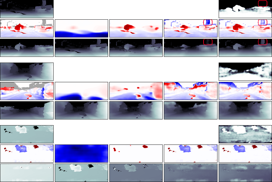
(a) Ground truth (b) Baseline
(c) Baseline + our losses (d) Ours (no attn; no GC)
(e) Ours (full)
Figure 6: Illustration of how the quality of the predictions changes as different components are added to the system. Each three
rows show an example, as follows: (a) Input inverse-depth and ground-truth error, and ground-truth inverse-depth. The shaded
areas in the ground-truth error represent missing data in the reference mesh. (b)–(d) Prediction and corrected inverse-depth.
(e): Attention mask, prediction, and corrected inverse-depth. The baseline model (b) only learns very rough predictions and is
unable to generalise well to the top viewpoint (last example). Our proposed losses help with generalisation across viewpoints,
but without skip connections in the network predictions are not very well localised (c). Our model (d); (e) makes well-localised
predictions. The attention mask removes some of the spurious predictions where there is no reference data (e). For example, the
highlighted background structure in the first example is removed when the attention mask is not used (d), while the attention
mask disables edits to that region of the input image (e).
This highlights the ability of our model to reduce gross
errors.
4.4 Ablation Study
To better understand how different components of our
model improve the learnt correction, we perform an
ablation study. The results in Table 4 show that our
proposed geometric consistency loss (rows with GC)
improves performance at all error scales.
The proposed attention mask (rows with attn) im-
proves the performance in the absence of geometric
consistency, but slightly limits the performance espe-
cially with larger errors. However, qualitatively (Fig-
ure 6), the attention mask allows us to better handle
missing training data (that is greyed out in the ground
truth column). In particular, surfaces are not spuri-
ously removed or added in those regions: the model
learns to mask those regions out of the correction and
keep them as they are.
4.5 Corrected Meshes
We demonstrate our method in practice by using the
corrected inverse-depth images to create new, cor-
rected reconstructions of the input meshes. Our model
effectively corrects missing surfaces, particularly on
the road, as illustrated in Figure 7. This results in
higher surface coverage of the original scene.
As is common with neural networks trained for
image regression, predictions can sometimes be too
smooth. While we address this by using skip connec-
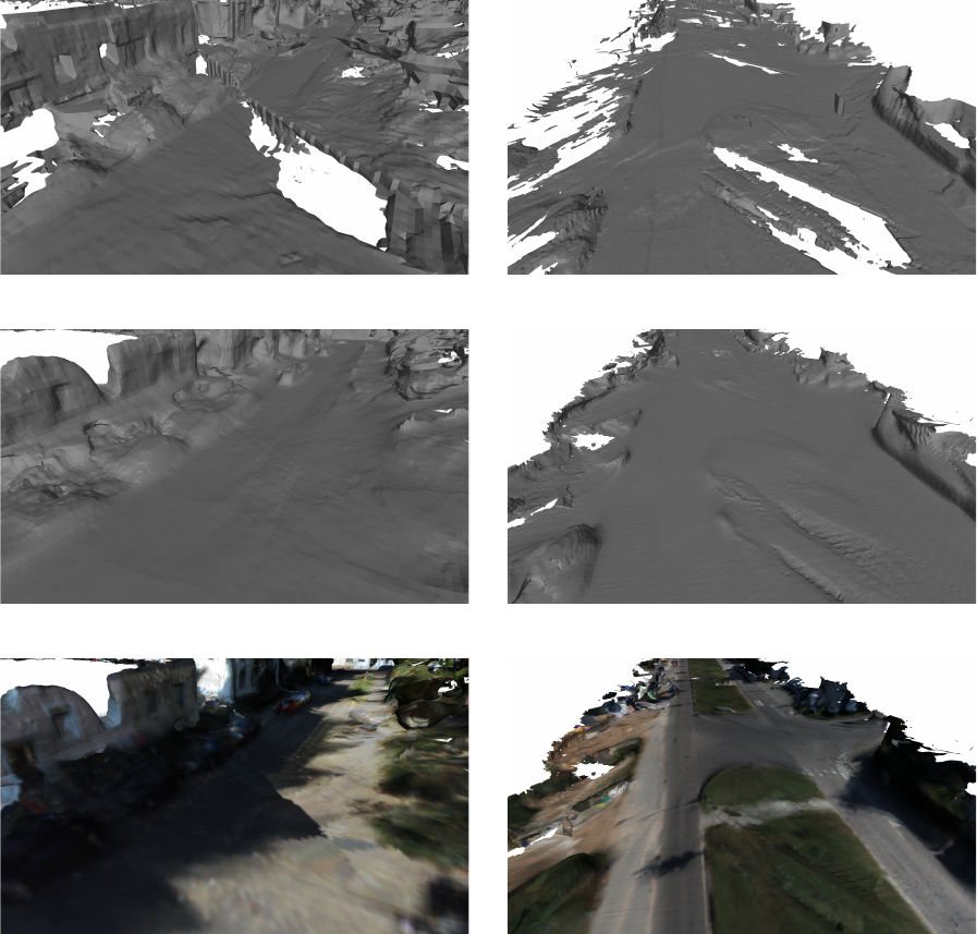
(a) Uncorrected mesh
(b) Corrected mesh
(c) Full colour reconstruction
Figure 7: Images of 3D reconstructions of KITTI sequence 00 (left) and 06 (right). (a) Shows the uncorrected meshes that our
network processes, built solely from a stereo camera. Note the large missing surfaces due to either poor lighting, or poorly
textured regions. Our model recovers the missing surfaces (b), providing a more complete reconstruction. (c) shows the
corrected meshes with colour copied from the uncorrected input. The models used for this illustration here are trained as
described in Section 4.3, so the corrected meshes are not part of the training data.
tions between the encoder and decoder of the network,
smoothness in predictions can still occur, especially
when there are no edges in the network input to guide
the output. This is not a problem when filling in closed
holes like the ones in the road, which have clear bound-
aries. However, for regions without clear boundaries,
such as the top of buildings, network predictions are
too smooth. This can be seen in both Figure 6 and
Figure 7.
5 CONCLUSION
In this paper we present a method for correcting gross
errors in dense 3D meshes. We extracted paired 2D
mesh features from two reconstructions and trained a
neural network to predict the difference in inverse-
depth between the two. We addressed the issue
of overly-smooth predictions with a U-Net architec-
ture and a loss-weighting mechanism that emphasises
edges. The geometric consistency of our predictions is
improved with a view-synthesis loss that targets incon-
sistencies. Our experiments show that the proposed
method reduces gross errors in inverse-depth views of
the mesh by up to 77.5%.
While in this paper we focus on correcting meshes
of urban scenes built from street-level sensors, our
method is generally applicable to environments with
strong priors that can be learnt from data.
ACKNOWLEDGEMENTS
The authors would like to acknowledge the support
of the UK’s Engineering and Physical Sciences Re-
search Council (EPSRC) through the Centre for Doc-
toral Training in Autonomous Intelligent Machines
and Systems (AIMS) Programme Grant EP/L015897/1.
Paul Newman is supported by EPSRC Programme
Grant EP/M019918/1.
REFERENCES
Bredies, K., Kunisch, K., and Pock, T. (2010). Total gener-
alized variation. SIAM Journal of Imaging Sciences,
3:4920–526.
Canny, J. F. (1986). A computational approach to edge
detection. IEEE Transactions on Pattern Analysis and
Machine Intelligence, PAMI-8:679–698.
Chambolle, A. and Pock, T. (2011). A first-order primal-
dual algorithm for convex problems with applications
to imaging. Journal of Mathematical Imaging and
Vision, 40(1):120–145.
Dharmasiri, T., Spek, A., and Drummond, T. (2019). ENG:
End-to-end neural geometry for robust depth and pose
estimation using CNNs. In Proceedings of the Asian
Conference on Computer Vision (ACCV), pages 625–
642.
Eldesokey, A., Felsberg, M., and Khan, F. S. (2018). Prop-
agating confidences through CNNs for sparse data re-
gression. In Proceedings of the British Machine Vision
Conference (BMVC).
Felzenszwalb, P. F. and Huttenlocher, D. P. (2012). Distance
transforms of sampled functions. Theory of Computing,
8:415–428.
Godard, C., Mac Aodha, O., and Brostow, G. J. (2017). Un-
supervised monocular depth estimation with left-right
consistency. In Proceedings of the IEEE International
Conference on Computer Vision and Pattern Recogni-
tion (CVPR).
He, K., Zhang, X., Ren, S., and Sun, J. (2016). Deep residual
learning for image recognition. In Proceedings of the
IEEE International Conference on Computer Vision
and Pattern Recognition (CVPR), pages 770–778.
Hua, J. and Gong, X. (2018). A normalized convolutional
neural network for guided sparse depth upsampling. In
Proceedings of the International Joint Conference on
Artificial Intelligence (IJCAI).
Jeon, J. and Lee, S. (2018). Reconstruction-based pairwise
depth dataset for depth image enhancement using CNN.
In Proceedings of the European Conference on Com-
puter Vision (ECCV).
Kingma, D. and Ba, J. (2015). Adam: A method for stochas-
tic optimization. In Proceedings of the International
Conference on Learning Representations (ICLR).
Klodt, M. and Vedaldi, A. (2018). Supervising the new with
the old: Learning SfM from SfM. In Proceedings of
the European Conference on Computer Vision (ECCV).
Knutsson, H. and Westin, C.-F. (1993). Normalized and
differential convolution: Methods for interpolation and
filtering of incomplete and uncertain data. In Proceed-
ings of the IEEE International Conference on Com-
puter Vision and Pattern Recognition (CVPR).
Kopf, J., Cohen, M. F., Lischinski, D., and Uyttendaele, M.
(2007). Joint bilateral upsampling. ACM Transactions
on Graphics, 26:96.
Kwon, H., Tai, Y.-W., and Lin, S. (2015). Data-driven depth
map refinement via multi-scale sparse representation.
In Proceedings of the IEEE International Conference
on Computer Vision and Pattern Recognition (CVPR),
pages 159–167.
Laina, I., Rupprecht, C., Belagiannis, V., Tombari, F., and
Navab, N. (2016). Deeper depth prediction with fully
convolutional residual networks. In Proceedings of the
IEEE International Conference on 3D Vision (3DV),
pages 239–248.
Ma, F. and Karaman, S. (2018). Sparse-to-dense: Depth pre-
diction from sparse depth samples and a single image.
In Proceedings of the IEEE International Conference
on Robotics and Automation (ICRA).
Mahjourian, R., Wicke, M., and Angelova, A. (2018). Un-
supervised learning of depth and ego-motion from
monocular video using 3D geometric constraints. In
Proceedings of the IEEE International Conference
on Computer Vision and Pattern Recognition (CVPR),
pages 5667–5675.
Matsuo, T., Fukushima, N., and Ishibashi, Y. (2013).
Weighted joint bilateral filter with slope depth compen-
sation filter for depth map refinement. In Proceedings
of the International Conference on Computer Vision
Theory and Applications (VISAPP).
Newcombe, R. A., Izadi, S., Hilliges, O., Molyneaux, D.,
Kim, D., Davison, A. J., Kohli, P., Shotton, J., Hodges,
S., and Fitzgibbon, A. W. (2011). KinectFusion: Real-
time dense surface mapping and tracking. In IEEE
International Symposium on Mixed and Augmented
Reality, pages 127–136.
Owen, A. B. (2007). A robust hybrid of lasso and ridge
regression. Contemporary Mathematics, 443:59–72.
Riegler, G., R
¨
uther, M., and Bischof, H. (2016). ATGV-Net:
Accurate depth super-resolution. In Proceedings of the
European Conference on Computer Vision (ECCV).
Ronneberger, O., Fischer, P., and Brox, T. (2015). U-Net:
Convolutional networks for biomedical image segmen-
tation. In Medical Image Computing and Computer
Assisted Intervention (MICCAI).
Shi, W., Caballero, J., Husz
´
ar, F., Totz, J., Aitken, A. P.,
Bishop, R., Rueckert, D., and Wang, Z. (2016). Real-
time single image and video super-resolution using
an efficient sub-pixel convolutional neural network.
In Proceedings of the IEEE International Conference
on Computer Vision and Pattern Recognition (CVPR),
pages 1874–1883.
Sobel, I. and Feldman, G. (1968). A 3
×
3 isotropic gradi-
ent operator for image processing. presented at the
Stanford Artificial Intelligence Project (SAIL).
Tanner, M., Pini
´
es, P., Paz, L. M., and Newman, P. (2015).
BOR
2
G: Building optimal regularised reconstructions
with GPUs (in cubes). In Proceedings of the Interna-
tional Conference on Field and Service Robotics (FSR),
Toronto, Canada.
Tanner, M., Pini
´
es, P., Paz, L. M., and Newman, P. (2016).
Keep geometry in context: Using contextual priors for
very-large-scale 3d dense reconstructions. In Robotics:
Science and Systems (RSS). Workshop on Geometry
and Beyond: Representations, Physics, and Scene Un-
derstanding for Robotics.
Tanner, M., S
˘
aftescu,
S
,
., Bewley, A., and Newman, P. (2018).
Meshed up: Learnt error correction in 3D reconstruc-
tions. In Proceedings of the IEEE International Con-
ference on Robotics and Automation (ICRA), Brisbane,
Australia.
Tomasi, C. and Manduchi, R. (1998). Bilateral filtering for
gray and color images. In Proceedings of the Interna-
tional Conference on Computer Vision (ICCV), pages
839–846.
Uhrig, J., Schneider, N., Schneider, L., Franke, U., Brox, T.,
and Geiger, A. (2017). Sparsity invariant CNNs. In
Proceedings of the IEEE International Conference on
3D Vision (3DV).
Ummenhofer, B., Zhou, H., Uhrig, J., Mayer, N., Ilg, E.,
Dosovitskiy, A., and Brox, T. (2017). DeMoN: Depth
and motion network for learning monocular stereo.
In Proceedings of the IEEE International Conference
on Computer Vision and Pattern Recognition (CVPR),
pages 5622–5631.
Zhang, Y. and Funkhouser, T. A. (2018). Deep depth com-
pletion of a single RGB-D image. In Proceedings of the
IEEE International Conference on Computer Vision
and Pattern Recognition (CVPR), pages 175–185.
Zhou, T., Brown, M., Snavely, N., and Lowe, D. G. (2017).
Unsupervised learning of depth and ego-motion from
video. In Proceedings of the IEEE International Con-
ference on Computer Vision and Pattern Recognition
(CVPR).
