A Hierarchical Loss for Semantic Segmentation

Bruce R. Muller

and William A. P. Smith

Department of Computer Science, University of York, York, U.K.

Keywords:

Semantic Segmentation, Class Hierarchies, Scene Understanding.

Abstract:

We exploit knowledge of class hierarchies to aid the training of semantic segmentation convolutional neural

networks. We do not modify the architecture of the network itself, but rather propose to compute a loss that is

a summation of classiﬁcation losses at different levels of class abstraction. This allows the network to differen-

tiate serious errors (the wrong superclass) from minor errors (correct superclass but incorrect ﬁnescale class)

and to learn visual features that are shared between classes that belong to the same superclass. The method

is straightforward to implement (we provide a PyTorch implementation that can be used with any existing

semantic segmentation network) and we show that it yields performance improvements (faster convergence,

better mean Intersection over Union) relative to training with a ﬂat class hierarchy and the same network

architecture. We provide results for the Helen facial and Mapillary Vistas road-scene segmentation datasets.

1 INTRODUCTION

The visual world is full of structure, from relation-

ships between objects to scenes and objects composed

of hierarchical parts. For example, at the most ab-

stract level, a road scene could be segmented into

three parts: ground plane, objects on the ground plane

and the sky. The next ﬁner level of abstraction might

differentiate the ground plane into road and pavement,

then the road into lanes, white lines and so on. Hu-

man perception exploits this structure in order to rea-

son abstractly without having to cope with the deluge

of information when all features and parts are consid-

ered simultaneously. Moreover, it is quite easy for a

human to describe this structure in a consistent way

and to reﬂect it in annotations or labels. It is therefore

surprising that the vast majority of work on learning-

based object recognition, object detection, semantic

segmentation and many other tasks completely ig-

nores this structure. Classiﬁcation tasks are usually

solved with a ﬂat class hierarchy, but in this paper

we seek to utilise this structure. Another motivation

is that there is often inhomogeneity between datasets

in terms of labelling. For example, the LFW parts

label database (Kae et al., 2013) segments face im-

ages into background, hair and skin, while the seg-

ment annotations (Smith et al., 2013) for the Helen

dataset (Le et al., 2012) deﬁne 11 segments. Util-

https://orcid.org/0000-0003-3682-9032

https://orcid.org/0000-0002-6047-0413

ising both datasets to train a single network, while

retaining the richness of the labels in the latter one,

is not straightforward. Depending on the applica-

tion, we may also wish to be able to vary the gran-

ularity of labels provided by the same network.

In this paper, we tackle the problem of semantic

segmentation and introduce the idea of hierarchical

classiﬁcation loss functions. The idea is very sim-

ple. Any existing semantic segmentation architecture

that outputs one logit per class per pixel (and which

would conventionally be trained using a single classi-

ﬁcation loss such as cross entropy) can compute a sum

of losses at each level of abstraction within the class

hierarchy. The beneﬁt is to differentiate serious errors

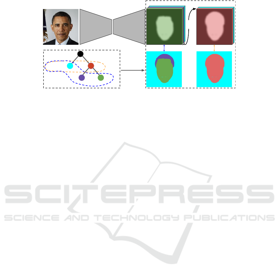
from less serious. In the toy example shown in Fig. 1,

a face/hair error would be penalised less severely than

a background/face error since both face and hair be-

long to the superclass head and so L

would not pe-

nalise the error. This encourages the network to learn

visual features that are shared between classes be-

longing to the same superclass, i.e. the knowledge

conveyed by the class hierarchy allows the network to

exploit regularity in appearance. Since coarser classi-

ﬁcation into fewer abstract classes is presumably sim-

pler than ﬁnescale classiﬁcation, it also means that the

learning process can naturally proceed in a coarse to

ﬁne manner, learning the more abstract classes earlier.

The approach is very simple to implement, requiring

only a few lines of code to compute the hierarchical

losses once the tree has been constructed.

260

Muller, B. and Smith, W.

A Hierarchical Loss for Semantic Segmentation.

DOI: 10.5220/0008946002600267

In Proceedings of the 15th International Joint Conference on Computer Vision, Imaging and Computer Graphics Theory and Applications (VISIGRAPP 2020) - Volume 4: VISAPP, pages

260-267

ISBN: 978-989-758-402-2; ISSN: 2184-4321

Any semantic

segmentation architecture

head

background

face

hair

0.3

0.4

0.3

0.7

Total loss = L

Class hierarchy

Hierarchical Loss Layer

p(c)

p(c

)

Figure 1: Overview of our idea. Given the output of any semantic segmentation architecture and a class hierarchy, we compute

losses for each level of abstraction within the hierarchy, inferring probabilities of superclasses from their children.

2 RELATED WORK

Semantic Segmentation. The state-of-the-art in se-

mantic segmentation has advanced rapidly in the last

5 years thanks to end-to-end learning with fully con-

volutional networks (Long et al., 2015). The ﬁeld is

large, so we provide only a brief summary here. A

landmark paper was SegNet (Badrinarayanan et al.,

2017) which utilised an encoder-decoder architec-

ture with skip connections with a novel unpooling

operation for upsampling. Wu et al. (Wu et al.,

2019) recently explored extensions of this architec-

ture. G

uc¸l

u et al. (G

uc¸l

u et al., 2017) perform fa-

cial semantic segmentation by augmenting a convo-

lutional neural network (CNN) with conditional ran-

dom ﬁelds and an adversarial loss. Ning et al. (Ning

et al., 2018) achieve very fast performance using hier-

archical dilation units and feature reﬁnement. Cur-

rent state-of-the-art facial segmentation is achieved

by Lin et al. (Lin et al., 2019) using a spatial fo-

cusing transform and a Mask R-CNN/Resnet-18-FPN

region-of-interest network for segmenting facial sub-

components into a whole. Rota Bul

o et al. (Rota Bul

et al., 2018) achieve state-of-the-art road scene se-

mantic segmentation performance. They combine a

DeepLabv3 head with a wideResNExt body and pro-

pose a special form of activated batch normalisation

which saves memory and allowing for a larger net-

work throughput. Zhao et al. (Zhao et al., 2017)

proposed Pyramid Scene Parsing Network (PSPNet)

which utilises a new architecture module to capture

contextual information. Chen et al. (Chen et al., 2018)

extend DeepLabv3 by adding a decoder module based

on atrous separable convolution. None of these meth-

ods exploit scene structure provided by class hierar-

chies.

Hierarchical Methods. Existing hierarchy-based

methods have focused on hierarchical architectures,

i.e. methods that speciﬁcally adapt the architecture of

the network to the speciﬁc hierarchy for a particular

task. This is typiﬁed by Branch-CNN (Zhu and Bain,

2017) and Hierarchical Deep CNN (Yan et al., 2015)

in which a network architecture is constructed to re-

ﬂect the classiﬁcation hierarchy. Luo et al. (Luo et al.,

2012) use face and component detections to constrain

face segmentation.

Deng et al. (Deng et al., 2014) encode class rela-

tionships in a Hierarchy and Exclusion (HEX) graph.

This enables them to reason probabilistically about la-

bel relations using a CRF. While very powerful, this

also makes inference on their model more expensive

and deﬁning a HEX graph requires richer information

than we use.

Srivastava and Salakhutdinov (Srivastava and

Salakhutdinov, 2013) similarly take a probabilistic

approach and attempt to learn a hierarchy as part of

the training process. This does not necessarily reﬂect

the semantic class structure but is rather chosen to op-

timise subsequent classiﬁcation performance. Again,

inference is more complex and expensive.

Meletis et al. (Meletis and Dubbelman, 2018) use

a restricted set of classiﬁers in a hierarchical fashion

on the output of a standard deep learning architecture

to harness differing levels of semantic description.

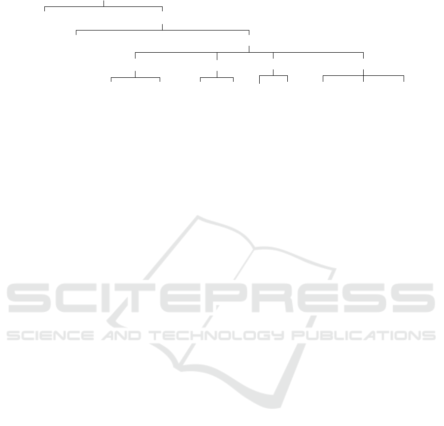
3 HIERARCHY DESIGN

Our approach requires a predeﬁned hierarchy, which

we assume is designed based on expert human knowl-

edge. In the case of objects composed of parts, this

is straightforward since the parts can naturally be de-

scribed hierarchically. For more general scenes this

may require speciﬁc domain knowledge in order to be

able to group related objects together into the same

A Hierarchical Loss for Semantic Segmentation

261

image

background

foreground

hair

face

eyebrows

right-eyebrow

left-eyebrow

eyes

right-eye

left-eye

skin

nose

face-skin

mouth

lower-lip

inner-mouth

upper-lip

Figure 2: Our hierarchy for the Helen segment classes. Note that the classes in the original dataset (Smith et al., 2013) are the

leaves in our hierarchy.

superclass. We emphasise two points. First, the prac-

tical effort of doing this is extremely low. We do not

require any new annotation of the training images,

there is simply a one off task to design a hierarchy

for the classes already used in the labelling. Second,

many existing datasets were annotated with a hierar-

chical class structure in mind (even if this is rarely

used). For example, the COCO-stuff dataset (Chen

et al., 2018) clusters each of the 172 classes into 11

abstract groups, providing a shallow hierarchy.

For the experiments in this paper we use two

datasets that represent each of the cases above. The

segment annotations (Smith et al., 2013) for the Helen

dataset (Le et al., 2012) are not provided with any hi-

erarchy. However, there is an obvious parts-based par-

titioning such that the classes used in the dataset cor-

respond to the leaves of a hierarchy tree (see Fig. 2).

To emphasise again: we do not need to relabel the

Helen annotations. We simply use the original anno-

tations in conjunction with the hierarchy. The sec-

ond case is the Mapillary Vistas road scene dataset.

This was originally designed with a hierarchical class

structure (see (Neuhold et al., 2017) for details) for

which some superclasses are based on clustering re-

lated objects (for example, the vehicle superclass).

4 HIERARCHICAL LOSS

Our method is based on computing a sum of classi-

ﬁcation losses over each level of abstraction within a

classiﬁcation hierarchy. In order to use the approach,

one simply needs a class hierarchy deﬁned by a tree

and a segmentation architecture that outputs a classi-

ﬁcation for each of the classes corresponding to leaf

nodes in the tree. In this section we describe our rep-

resentation and the hierarchical losses.

Tree-based Representation. We represent our

class hierarchy using a tree (V, E), with V =

, . . . , v

} the set of vertices and E ⊂ V ×V the set

of ordered edges such that (v

, v

) ∈ E encodes that

is a parent of v

. We assume that the ﬁrst m nodes

correspond to leaves in the tree, i.e. @ v

∈ V, (v

, v

) ∈

E ⇒ 1 ≤ i ≤ m. These nodes correspond to the ﬁnest

scale classes. If (v

, v

) ∈ E then v

is a more gen-

eral, more abstract, superclass of v

. The label for a

pixel, c, should be at the ﬁnest level of classiﬁcation,

i.e. c ∈ {1, . . . , m}.

We deﬁne depth(v

) to mean the number of edges

between vertex v

and the root node. Hence, the depth

of the tree is given by D

max

= max

depth(v

). We

deﬁne ancestor(v

, v

) to be true if v

is an ancestor of

, i.e. that v

is a superclass of v

and false otherwise.

Inferring Coarse Classes from Fine. We assume

that the segmentation CNN outputs one logit, x

, per

pixel per leaf node, i.e. the output of the network is

of size H × W × m. Hence, the probability, p

, as-

sociated with node i can be computed by applying the

softmax function, σ : R 7→ [0, 1], to x

. The probability

associated with non-leaf nodes is deﬁned recursively

by summing the probabilities of its children until leaf

nodes are reached:







σ(x

) if 1 ≤ i ≤ m

∑

)∈E

otherwise

(1)

Note that any summation is over a subset of leaf-

nodes whose total sum is one so any p

is ≤ 1.

Depth Dependent Losses. The appropriate label

varies depending on the level of abstraction, i.e. the

depth considered in the tree. We deﬁne the correct

class at a depth d ∈ {0, . . . , D

max

} to be:

(

c if depth(v

) ≤ d

i, depth(v

) = d ∧ anc(v

, v

) otherwise

(2)

where anc(v

, v

) denotes the ancestor of nodes v

and

. The classiﬁcation loss at depth d is computed us-

ing the negative log loss as L

= −log(p

). Note that

= 0. The total hierarchical loss is then a summa-

tion over all depths in the tree: L =

∑

max

d=0

VISAPP 2020 - 15th International Conference on Computer Vision Theory and Applications

262

background

foreground

hair

face

mouth

upper_lip

inner_mouth

lower_lip

skin

face_skin

nose

eyes

left_eye

right_eye

eyebrows

left_eyebrow

right_eyebrow

precomputed_hierarchy_list = [

[ [background],[hair],[upper_lip],[inner_mouth],[lower_lip],[face_skin],

[nose],[left_eye],[right_eye],[left_eyebrow],[right_eyebrow] ],

[ [background],[hair],[upper_lip],[inner_mouth],[lower_lip],

[face_skin,nose],[left_eye,right_eye],[left_eyebrow,right_eyebrow] ],

[ [background],[hair],[upper_lip,inner_mouth,lower_lip,face_skin,nose,

left_eye,right_eye,left_eyebrow,right_eyebrow] ],

[ [background],[hair,upper_lip,inner_mouth,lower_lip,face_skin,nose,

left_eye,right_eye,left_eyebrow,right_eyebrow] ] ]

Figure 3: Class hierarchy implementation example for the hierarchy in Fig. 2. In our implementation the classiﬁcation

hierarchy is provided as a text ﬁle (left). From this, we precompute lists of leaf nodes (right) for each abstraction depth

corresponding to the summations required for computing internal node probabilities (e.g. Fig. 1 bottom-left: hair and face

class probabilities infer a value of 0.7 for the abstract class head). The four sub-lists in precomputed hierarchy list

correspond to the four abstraction depths for the hierarchy depicted in Fig. 2.

5 IMPLEMENTATION

In this section we describe implementation details for

our hierarchical loss function. Our implementation is

written using standard PyTorch layers and we make it

publicly available

in a form that is easy to integrate

with any existing semantic segmentation architecture.

We also explain how to ensure numerical stability in

the computation of these losses.

Tree Structure. The hierarchical class structure is

provided as a text ﬁle using indentation to signify par-

ent/child relationships. For example the Helen hierar-

chy we use in Fig. 2 is written as a text ﬁle as shown in

Fig. 3 (left). Loading the text ﬁle, we internally store

the tree as a structure of linked python objects called

nodes. Each leaf-node in the hierarchy represents a

class in our dataset and encapsulates an integer rep-

resenting the channel it will use in the output of the

neural network. Additionally we ensure to keep con-

sistent the integer numbering between class labels in

the training data and python hierarchical leaf-nodes.

To implement our hierarchical loss, we precom-

pute lists representing the set of leaf node classes

that belong to each superclass (see Fig. 3 (right)

for an example on the Helen dataset). We may

think of the hierarchy in terms of various levels of

abstraction. For example, the hierarchy in Fig. 1

has two abstraction levels: the base level where

we take all leaf-nodes, and the level up where we

have background and head (which is inferred from

github.com/brucemuller/HierarchicalLosses

hair and face). In that case we could precom-

pute the lists [ [background], [hair], [face]]

and [[background], [hair, face]] for the base

and more abstract level respectively. For our Helen

dataset we have four levels of abstraction as shown

by the hierarchy in Figures 2 and 3.

It is important to note that every leaf class will

contribute to the same number of losses regardless of

the hierarchical depth, and we are not assigning dif-

ferent weights to different classes based on how deep

they are in the class hierarchy.

To illustrate the simplicity and generalisability of

our idea, we have included the code snippet in Listing

1. Note that for clarity, we ignore the numerical sta-

bility issues (discussed below) in this snippet. Here

we illustrate exactly how the output of any neural net-

work semantic segmentation classiﬁcation layer can

be processed to compute hierarchical loss from an

easily designed semantic hierarchy. The output from

the CNN is deep copied for each depth in the tree to

compute the separate level losses.

Each level loss list represents the branches with

which we need to sum probabilities. We use the level

loss list for a particular abstraction level to extract the

softmaxed CNN output channels to be summed over

(lines 7 to 12 of Listing 1). Every summed slice of

a branch is inserted into each channel associated with

that branch for ease of implementation (lines 19 and

20 of Listing 1). While this step duplicates probabil-

ity slices in summed probabilities for a particular

abstraction level, it allows us to easily pass into any

PyTorch loss. Finally to compute the loss for each ab-

A Hierarchical Loss for Semantic Segmentation

263

1 p r o b a b i l i t i e s = s o f t m a x ( c n n o u t p u t , dim = 1 ) ; l o s s = 0

3 f o r l e v e l l o s s l i s t i n p r e c o m p u t e d h i e r a r c h y l i s t

5 p r o b a b i l i t i e s t o s u m = p r o b a b i l i t i e s . c l o n e ( )

6 s u m m e d p r o b a b i l i t i e s = p r o b a b i l i t i e s t o s u m

7 f o r b r a nc h i n l e v e l l o s s l i s t :

9 # E x t r a c t t h e r e l e v a n t p r o b a b i l i t i e s a c c o r d i n g t o a b ra nc h i n o ur h i e r a r c h y .

10 b r a n c h p r o b s = t o r c h . F l o a t T e n s o r ( )

11 f o r c h a nn e l i n b r a n ch :

12 b r a n c h p r o b s = t o r c h . c a t ( ( b r a n c h p ro b s , p r o b a b i l i t i e s t o s u m [ : , c h a n n e l , : , : ] . u ns qu ee ze ( 1 ) ) , 1 )

14 # Sum t h e s e p r o b a b i l i t i e s i n t o a s i n g l e s l i c e ; t h i s i s h i e r a r c h i c a l i n f e r e n c e .

15 s u m m e d t r e e b r a n c h s l i c e = b r a n c h p r o b s . sum (1 , k e epdim =Tr ue )

17 # I n s e r t i n f e r r e d p r o b a b i l i t y s l i c e i n t o ea c h c h a n n e l o f s u m m e d p r o b a b i l i t i e s g iv e n by b ra n c h .

18 # T hi s d u p l i c a t e s p r o b a b i l i t i e s f o r e a s y p a s s i n g t o s t a n d a r d l o s s f u n c t i o n s su ch a s n l l l o s s .

19 f o r c h a nn e l i n b r a n ch :

20 s u m m e d p r o b a b i l i t i e s [ : , c h an n e l : ( c h a nn e l +1) , : , : ] = s u m m e d t r e e b r a n c h s l i c e

22 l e v e l l o s s = n l l l o s s ( l o g ( s u m m e d p r o b a b i l i t i e s ) , t a r g e t )

23 l o s s = l o s s + l e v e l l o s s

24 r e t u r n ( l o s s )

Listing 1: PyTorch snippet for computing the inferred probabilities at the abstraction levels in our hierarchy. The hierarchy

of classes is represented by level loss list, which is a list of lists composed of integers representing our branching

classes.

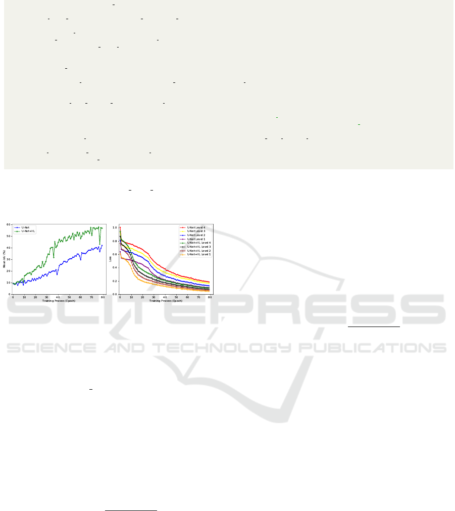
Figure 4: Training behaviour versus epoch on the Helen

dataset. Left: Mean IOU. In both cases we show results

trained with vanilla (U-Net) and hierarchical (U-Net+HL)

losses. Right: Classiﬁcation loss for each depth D = 1..4.

straction level, we take the log of the summed proba-

bility tensor, which is passed to the negative log like-

lihood loss layer (nll loss) along with labels.

Numerical Stability. Evaluating cross entropy

(log) loss of a probability computed using softmax

is numerically unstable and can easily lead to over-

ﬂow or underﬂow. In most implementations, this is

circumvented using the “log-sum-exp trick” (Murphy,

2006) derived from the identity exp(x) = exp(x − b +

b) = exp(x − b) exp(b):

L = − log p

= − log

exp(x

)

∑

j=1

exp(x

)

− x

+ b + log

∑

j=1

exp(x

− b), (3)

where b = max

i∈{1,...,n}

is chosen so that the maxi-

mum exponential has value one and thus avoids over-

ﬂow, while at least one summand will avoid under-

ﬂow and hence avoid taking a logarithm of zero.

Our hierarchical classiﬁcation losses involve com-

puting log losses on internal nodes in the class hierar-

chy tree. The probabilities in these nodes are in turn

formed by summing probabilities computed by apply-

ing softmax to CNN outputs. This leads to evaluation

of losses of the form −log(

∑

i∈C

) where C is the set

of leaf nodes contributing to the superclass. This can

be made numerically stable by double application of

the log-sum-exp trick:

L = − log

∑

i∈C

= − log

∑

i∈C

exp(x

)

∑

j=1

exp(x

)

b + log

∑

j=1

exp(x

− b) − b

− log

∑

i∈C

exp(x

− b

(4)

b is deﬁned as before while b

= max

i∈C

. The use

of two different shifts for the two logarithm terms is

required to avoid underﬂow when b

 b.

6 EXPERIMENTS

We seek to investigate the relative performance gain

in using the hierarchical loss versus training simply

on a ﬂat hierarchy. To this end, in our experiments we

train two networks for each task. One is a “vanilla”

U-net (Ronneberger et al., 2015), the other is exactly

the same U-net architecture but trained with hierarchi-

cal loss (referred to as U-net+HL). We train U-Net/U-

Net+HL models simultaneously such that they receive

identical data input at each iteration. Note that we

do not seek nor achieve state-of-the-art performance.

A more complex architecture, problem-speciﬁc tun-

ing and so on would lead to improved performance

but our goal here is to assess relative performance

VISAPP 2020 - 15th International Conference on Computer Vision Theory and Applications

264

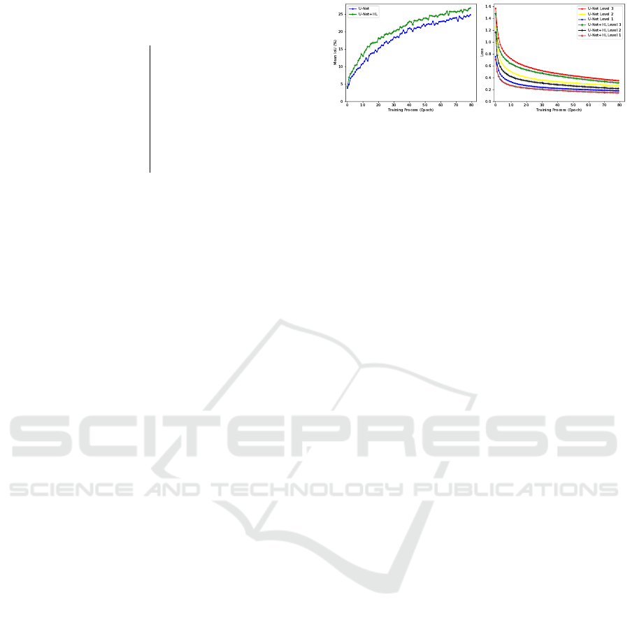
Table 1: Mean and class IOU (%) on Helen and Vistas (sub-

set selected) datasets at training convergence.

Helen Dataset Vistas Dataset

Class U-Net U-Net+HL Class U-Net U-Net+HL

Background 92.04 92.653 Car 80.35 80.91

Face skin 86.53 87.04 Terrain 54.21 56.07

Left eyebrow 63.12 62.68 Lane Marking 49.14 51.69

Right eyebrow 63.65 64.25 Building 77.31 79.67

Left eye 63.98 67.81 Road 82.31 82.69

Right eye 64.92 72.72 Trash Can 5.38 18.63

Nose 84.05 82.55 Manhole 2.25 16.96

Upper lip 52.88 56.48 Catch Basin 1.58 13.59

Inner mouth 62.17 67.94 Snow 56.97 71.46

Lower lip 65.64 67.92 Person 39.23 48.3

Hair 65.41 66.11 Water 29.87 16.1

Mean 69.49 71.65 Mean 24.74 26.51

gain using a simple baseline architecture. Networks

use Kaiming uniform initialisation with the same ran-

dom seed (to equally initialise vanilla and hierarchi-

cally trained networks). Pre-training is not utilised.

We use Stochastic Gradient Decent with a learning

rate of 0.01 and a batch size of 5 (due to memory

constraints). During training, images/labels were ran-

domly square-cropped using the shortest dimension

and re-sized to 256

. The only further augmentation

used was random ﬂipping (p = 0.5).

Datasets. For experimenting with hierarchical

losses on segmentation we chose two very different

datasets: the Helen (Le et al., 2012) facial dataset and

Mapillary’s Vistas (Neuhold et al., 2017) road scene

dataset. The Helen dataset covers a wide variety

of facial types (age, ethnicity, colour/grayscale,

expression, facial pose), originally built for facial

feature localisation (Le et al., 2012). We use an

augmented Helen (Smith et al., 2013) dataset with

semantic segmentation labels. Helen contains

2000, 230 and 100 images/annotations for training,

validation and testing respectively, for 11 classes

(10 facial and background, see Tab. 1(left)). It

should be noted that the ground truth annotations are

occasionally inaccurate, particularly for hair which

makes it challenging to learn. The road scene Vistas

dataset (Neuhold et al., 2017) is composed of 25000

images/annotations (18000 training, 2000 validation,

5000 testing), with 66 classes. As Vistas contains too

many classes to easily illustrate we have chosen only

a representative subset in Tab. 1 (right) which show

most signiﬁcant difference in performance and given

the mean over all classes. Further, our intention is

to indicate the performance improvement by using

hierarchical learning, rather than to compare between

datasets. The Vistas hierarchy is three levels deep,

contains 66 leaf nodes, and 11 internal nodes.

Results. Fig. 4 (right) shows losses for each ab-

straction depth of the class hierarchy for the He-

len experiment. Note that the deeper loss is always

Figure 5: Training behaviour on Vistas. Left: mean IOU

versus epoch. Right: classiﬁcation loss for each abstraction

depth D = 1..3 versus epoch. We show results trained with

vanilla (U-Net) and hierarchical (U-Net+HL) loss.

larger than a shallower one, suggesting that our hier-

archically trained method signiﬁcantly beneﬁts from

the hierarchical structure in the class labels, partic-

ularly in the early phase of training, learning much

faster than the vanilla model. Fig. 4 (left) illus-

trates the mean Intersection over Union (IOU) during

training. Performance gain is most signiﬁcant post

epoch 35 and can be observed in the qualitative re-

sults from Fig. 6. At performance convergence we

observe some qualitative differences between the hi-

erarchically trained network and the vanilla. For ex-

ample, in Fig. 6 U-net+HL predictions at epoch 200

have somewhat less hair artefacts, while the 1st exam-

ple shows improvement over a difﬁcult angled facial

pose. Epoch 50 results clearly show faster conver-

gence.

For Vistas, the IOU performance gain is less no-

table than on Helen, but we show the hierarchi-

cally trained model outperforming the vanilla model

in both level losses and mean IOU (Fig. 5 and

Tab. 1(right)). The qualitative results in Fig. 7 illus-

trate predictions for both methods at epoch 1 and 80.

Most interestingly, after 1 epoch the hierarchically

trained model is able to classify correctly a signiﬁ-

cant proportion of lane-markings whereas the vanilla

trained model cannot, showing how quickly our hi-

erarchical model is learning. Relative to the vanilla

model, our hierarchically trained model achieves a

3% and 7% relative improvement for Helen and Vis-

tas respectively (see Tab. 1).

7 CONCLUSIONS

Our results illustrate the great potential of using losses

that encourage semantically similar classes within a

hierarchy to be classiﬁed close together, where the

model parameters are guided towards a solution not

only better quantitatively, but faster in training than

using a standard loss implementation. We speculate

that the hierarchically trained models perform better

due to learning more robust features from visually

A Hierarchical Loss for Semantic Segmentation

265

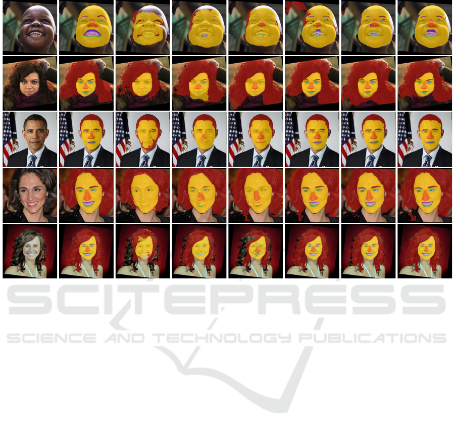
Input Ground Truth 30 Epochs 50 Epochs 200 Epochs

U-net U-net+HL U-net U-net+HL U-net U-net+HL

Figure 6: Prediction comparisons on the Helen dataset. From left to right: raw input image, ground truth annotation, vanilla

trained U-Net prediction at 30 epochs, hierarchically trained U-Net prediction at 30 epochs , vanilla trained U-Net prediction at

50 epochs, hierarchically trained U-Net prediction at 50 epochs, vanilla trained U-Net prediction at 200 epochs, hierarchically

trained U-Net prediction at 200 epochs.

similar classes which are close within the tree struc-

ture. The hierarchy is providing the network with

more information (e.g. a pixel belongs to an eye-brow,

which belongs to a face and so on), which can be

exploited to learn shared and more robust features.

There is a possible link to metric learning here where,

rather than positive and negative class labels, we are

provided with classes that can be more or less simi-

lar within a hierarchy. A particular advantage of this

work is its generality and self-contained nature allows

the possibility of plugging this hierarchical loss on the

end of any deep learning architecture. Taking advan-

tage of the hierarchical cues readily apparent to us can

help train a deep network faster and with greater ac-

curacy. Moreover any hierarchical structure can be

provided to help train your model. We also contribute

a numerically stable formulation for computing log

and softmax of a network output separately, a neces-

sity for summing probabilities according to a hierar-

chical structure. Future work could include learning

the hierarchy itself which best solves your task. Addi-

tionally we would like to use our ideas to construct a

level of abstraction segmenter for tree based labels on

hierarchically trained models. Ability to extract seg-

mentations at multiple levels in a hierarchy describing

your data is quite useful, intuitive and is not some-

thing commonly achieved by semantic segmentation

solvers in the current community.

REFERENCES

Badrinarayanan, V., Kendall, A., and Cipolla, R. (2017).

Segnet: A deep convolutional encoder-decoder archi-

tecture for image segmentation. IEEE TPAMI.

Chen, L.-C., Zhu, Y., Papandreou, G., Schroff, F., and

Adam, H. (2018). Encoder-decoder with atrous sep-

arable convolution for semantic image segmentation.

In Proc. ECCV, pages 801–818.

Deng, J., Ding, N., Jia, Y., Frome, A., Murphy, K., Bengio,

S., Li, Y., Neven, H., and Adam, H. (2014). Large-

scale object classiﬁcation using label relation graphs.

In Proc. ECCV, pages 48–64.

uc¸l

u, U., G

uc¸l

urk, Y., Madadi, M., Escalera, S., Bar

X., Gonz

alez, J., van Lier, R., and van Gerven,

M. A. (2017). End-to-end semantic face segmenta-

tion with conditional random ﬁelds as convolutional,

recurrent and adversarial networks. arXiv preprint

arXiv:1703.03305.

VISAPP 2020 - 15th International Conference on Computer Vision Theory and Applications

266

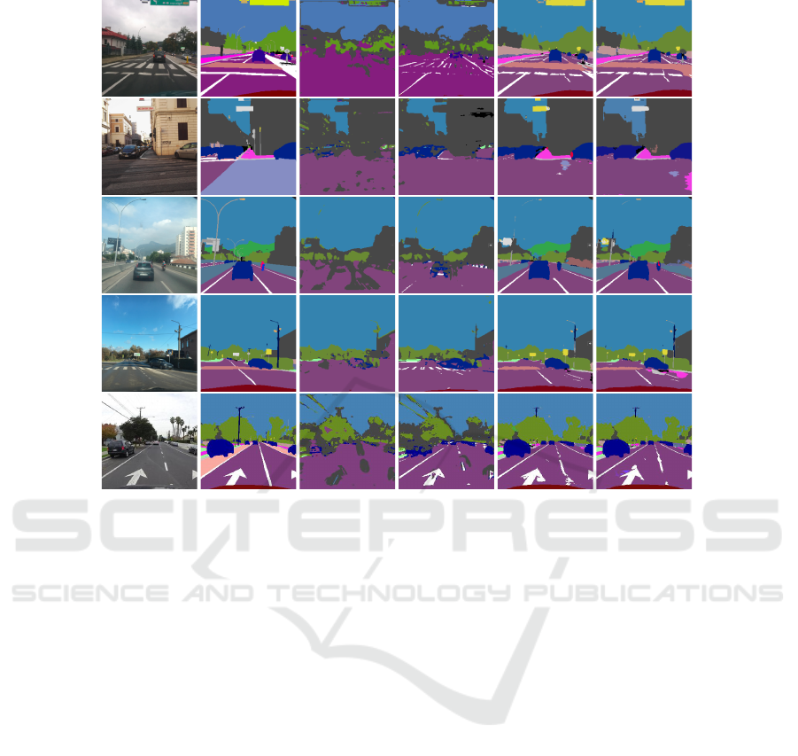
Input Ground truth 1 epoch 80 epochs

U-net U-net+HL U-net U-net+HL

Figure 7: Qualitative comparisons on Vistas. From left to right: raw input image, ground truth annotation, vanilla trained

U-Net prediction at 1 epoch, hierarchically trained U-Net prediction at 1 epoch, vanilla trained U-Net prediction at 80 epochs,

hierarchically trained U-Net prediction at 80 epochs.

Kae, A., Sohn, K., Lee, H., and Learned-Miller, E. (2013).

Augmenting crfs with boltzmann machine shape pri-

ors for image labeling. In Proc. CVPR, pages 2019–

2026.

Le, V., Brandt, J., Lin, Z., Bourdev, L., and Huang, T. S.

(2012). Interactive facial feature localization. In Proc.

ECCV, pages 679–692.

Lin, J., Yang, H., Chen, D., Zeng, M., Wen, F., and Yuan, L.

(2019). Face parsing with roi tanh-warping. In Proc.

CVPR, pages 5654–5663.

Long, J., Shelhamer, E., and Darrell, T. (2015). Fully con-

volutional networks for semantic segmentation. In

Proc. CVPR, pages 3431–3440.

Luo, P., Wang, X., and Tang, X. (2012). Hierarchical

face parsing via deep learning. In Proc. CVPR, pages

2480–2487. IEEE.

Meletis, P. and Dubbelman, G. (2018). Training of convo-

lutional networks on multiple heterogeneous datasets

for street scene semantic segmentation. In IVS (IV).

Murphy, K. P. (2006). Naive bayes classiﬁers. Technical

Report 18, University of British Columbia.

Neuhold, G., Ollmann, T., Rota Bulo, S., and Kontschieder,

P. (2017). The mapillary vistas dataset for semantic

understanding of street scenes. In Proc. ICCV, pages

4990–4999.

Ning, Q., Zhu, J., and Chen, C. (2018). Very fast seman-

tic image segmentation using hierarchical dilation and

feature reﬁning. Cogn. Comput., 10(1):62–72.

Ronneberger, O., Fischer, P., and Brox, T. (2015). U-net:

Convolutional networks for biomedical image seg-

mentation. In Proc. MICCAI, pages 234–241.

Rota Bul

o, S., Porzi, L., and Kontschieder, P. (2018).

In-place activated batchnorm for memory-optimized

training of dnns. In Proc. CVPR, pages 5639–5647.

Smith, B. M., Zhang, L., Brandt, J., Lin, Z., and Yang, J.

(2013). Exemplar-based face parsing. In Proc. CVPR,

pages 3484–3491.

Srivastava, N. and Salakhutdinov, R. R. (2013). Discrimina-

tive transfer learning with tree-based priors. In Proc.

NIPS, pages 2094–2102.

Wu, Z., Shen, C., and Van Den Hengel, A. (2019). Wider or

deeper: Revisiting the resnet model for visual recog-

nition. Pattern Recognition, 90:119–133.

Yan, Z., Zhang, H., Piramuthu, R., Jagadeesh, V., DeCoste,

D., Di, W., and Yu, Y. (2015). Hd-cnn: hierarchical

deep convolutional neural networks for large scale vi-

sual recognition. In Proc. ICCV, pages 2740–2748.

Zhao, H., Shi, J., Qi, X., Wang, X., and Jia, J. (2017). Pyra-

mid scene parsing network. In Proc. CVPR, pages

2881–2890.

Zhu, X. and Bain, M. (2017). B-cnn: Branch convolutional

neural network for hierarchical classiﬁcation. arXiv

preprint arXiv:1709.09890.

A Hierarchical Loss for Semantic Segmentation

267