
Variational Inference of Dirichlet Process Mixture using Stochastic
Gradient Ascent
Kart-Leong Lim
Nanyang Technological University, 50 Nanyang Ave 639788, Singapore
Keywords:
Bayesian Nonparametrics, Dirichlet Process Mixture, Stochastic Gradient Ascent, Fisher Information.
Abstract:
The variational inference of Bayesian mixture models such as the Dirichlet process mixture is not scalable to
very large datasets, since the learning is based on computing the entire dataset each iteration. Recently, scalable
version notably the stochastic variational inference, addresses this issue by performing local learning from
randomly sampled batches of the full dataset or minibatch each iteration. The main problem with stochastic
variational inference is that it still relies on the closed form update in variational inference to work. Stochastic
gradient ascent is a modern approach to machine learning and it is widely deployed in the training of deep
neural networks. It has two interesting properties. Firstly it runs on minibatch and secondly, it does not rely
on closed form update to work. In this work, we explore using stochastic gradient ascent as a baseline for
learning Bayesian mixture models such as Dirichlet process mixture. However, stochastic gradient ascent
alone is not optimal for learning in terms of convergence. Instead, we turn our focus to stochastic gradient
ascent techniques that use decaying step-size to optimize the convergence. We consider two methods here.
The commonly known momentum approach and the natural gradient approach which uses an adaptive step-
size through computing Fisher information. We also show that our new stochastic gradient ascent approach
for training Dirichlet process mixture is compatible with deep ConvNet features and applicable to large scale
datasets such as the Caltech256 and SUN397. Lastly, we justify our claims when comparing our method to an
existing closed form learner for Dirichlet process mixture on these datasets.
1 INTRODUCTION
A common task in Dirichlet process mixture (DPM)
is to automatically estimate the number of classes to
represent a dataset (a.k.a model selection) and clus-
ter samples accordingly in area such as image pro-
cessing, video processing and natural language pro-
cessing. The variational inference (VI) of DPM (Blei
et al., 2006; Bishop, 2006) is mainly based on closed
form coordinate ascent learning where it iteratively
repeats its computational task (or algorithm) on the
entire sequence of dataset samples each iteration, also
known as batch learning. (Blei et al., 2003; Kuri-
hara and Welling, 2009; Bishop, 2006), Scalable
algorithms of VI also allows DPM to scale up to
larger dataset at fractional cost. Due to the recent
paradigm shift towards deep ConvNet (Krizhevsky
et al., 2012; He et al., 2016) and deep generative net-
works (Kingma and Welling, 2014; Goodfellow et al.,
2014), it is very rare to find newer works focusing
on scalable DPM. Unlike DPM, deep ConvNet and
deep autoencoder do not specifically deal with model
selection. The more recent work addressing scalable
DPM or scalable Bayesian nonparametrics in general
is the stochastic variational inference (SVI) (Hoffman
et al., 2013; Paisley et al., 2015; Fan et al., 2018).
It is based on stochastic optimization (Robbins and
Monro, 1985) where it repeats its computational task
on a smaller set of randomly drawn samples each
iteration (or minibatch learning). This allows the
algorithm to see the entire dataset especially large
datasets when sufficient iterations has passed. SVI
was demonstrated on models with complex Bayesian
posteriors such as the hierarchical Dirichlet process
mixture (Hoffman et al., 2013) and on large datasets
as large as 3.8M documents and 300 topics. However,
SVI do not involve actual computation of gradient as-
cent. Instead, SVI fundamentally rely on closed form
coordinate ascent for learning. Also, the rate of step-
size decay in SVI is fixed and the optimal value is
usually unknown. This means that SVI cannot adapt
its step-size value according to the statistics of the
minibatch randomly drawn each iteration. Tradition-
ally, variational inference and stochastic gradient as-
Lim, K.
Var iational Inference of Dirichlet Process Mixture using Stochastic Gradient Ascent.
DOI: 10.5220/0008944300330042
In Proceedings of the 9th International Conference on Pattern Recognition Applications and Methods (ICPRAM 2020), pages 33-42
ISBN: 978-989-758-397-1; ISSN: 2184-4313
Copyright
c
2022 by SCITEPRESS – Science and Technology Publications, Lda. All rights reserved
33

cent are mutually exclusive. Recently, stochastic gra-
dient ascent (SGA) with constant step-size has been
discussed for VI in (Mandt et al., 2017). In a stochas-
tic or noisy setting (i.e. randomly drawn minibatch
samples), SGA with constant step-size alone may not
be efficient. There is a requirement for a decaying
step-size to ensure convergence in SGA. This is to
avoid SGA bouncing around the optimum of the ob-
jective function (Robbins and Monro, 1985).
When considering what are the current issues with
variational inference:
The main problems with VI (Blei et al., 2006) are:
a) Batch learning is slow.
b) Require analytical solution.
The main problems with SVI (Hoffman et al., 2013)
are:
b) Require analytical solution.
c) Fixed step-size decay for closed form learn-
ing.
The main problem with constant step-size SGA
(Mandt et al., 2017) is:
d) Constant step-size for SGA learning.
In this work, our goal is to learn a DPM to automat-
ically compute the number of clusters to represent
a dataset. We also seek to address the above prob-
lems in (a,b,c,d) by using SGA as a scalable algo-
rithm for DPM (in terms of CPU time) while seeking
to achieve at least on-par performance (i.e. cluster-
ing and model selection) with traditional VI. In order
to to achieve that, we turn our focus to stochastic op-
timization techniques that use decaying step-size to
optimize the learning in SGA. Instead of fixing the
rate of decay in SGA such as in the momentum ap-
proach, natural gradient (Amari, 1998) can provides
an adaptive step-size for SGA using Fisher informa-
tion. This is possible as directional search employ-
ing Fisher information in gradient ascent is akin to
directional search along the curvature of the objective
(variational posterior).
We test the performance of our proposed learner
on large class dataset such as Caltech256 and
SUN397 and obtained significant improvement over
VI. To the best of our knowledge, it is very rare to
find DPM task carried out on large scale image clas-
sification dataset i.e. large class sizes (397) and large
dataset (108K) such as Caltech256 and SUN397. The
experiments also confirmed that our proposed meth-
ods can handle large dimensional features (4096) such
as deep ConvNet features.
The novel contributions in this work are:
i) Avoid analytical solution.
ii) Adaptive step-size decay.
iii) Lower cost without sacrificing perfor-
mance.
This paper is organized as follows: Firstly, we present
a new technique based on constant step-size SGA to
take over VI for training a DPM. In order to have a
decreasing step-size effect, we smoothen the estima-
tion of SGA using the momentum approach. Thirdly,
instead of fixing the rate of step-size decay in the
momentum approach, we propose another alternative
by applying Fisher information to SGA, which adap-
tively learns a step-size decay from the variational
posterior, each iteration. We reported experimental
results on six datasets including the more challenging
Caltech256 and SUN397 for our DPM task. We first
compare the computational cost and the performance
of the proposed SGA to VI. Lastly, we compare our
method with state-of-the-arts methods for DPM.
1.1 Related Works
The use of SGA to perform VI is certainly not new.
We call these works as SGA-VI (Ranganath et al.,
2014; Paisley et al., 2012; Kingma and Welling, 2014;
Welling and Teh, 2011; Rezende and Mohamed,
2015). The key idea of SGA-VI is to take the gradient
of the evidence lower bound (ELBO) with a step size
for updating corresponding VI parameters. Some no-
table works in this area include the black box VI (Ran-
ganath et al., 2014), VI with stochastic search (Pais-
ley et al., 2012) and the stochastic gradient variational
Bayes (Kingma and Welling, 2014). An emphasis in
these works (e.g. black box VI) is the use of Monte
Carlo integration to approximate the expectation of
the ELBO. There are two advantages. Firstly, there is
no need to constrain the learning of variational pos-
teriors expectation to analytical solution. Secondly,
MCMC approximated solutions lead to true poste-
riors at the expense of greater computational cost.
However, most works usually demonstrated SGA-VI
on non-DPM related task such as the logistic regres-
sion(Welling and Teh, 2011; Mandt et al., 2017; Pais-
ley et al., 2012). Non-DPMs do not deal with in-
complete data or cluster label issue. Thus, the learn-
ing of the SGA-VI (Ranganath et al., 2014; Paisley
et al., 2012; Kingma and Welling, 2014; Welling and
Teh, 2011) described above are more suitable to rel-
atively simpler parameter inference problems. Also,
these works on SGA-VI were mainly demonstrated
on datasets with smaller datasets of 10 classes with
60K image sizes such as MNIST. In this paper we tar-
get BNP task of up to 108K images with 397 object
classes and high dimensions features of 4096 using
VGG16 pretrained on ImageNet and Place205. Our
work also falls under the SGA-VI category. Instead
ICPRAM 2020 - 9th International Conference on Pattern Recognition Applications and Methods
34

of Monte Carlo integration, we use the Maximum a
posterior (MAP) estimate for approximating the ex-
pectation of the ELBO for simplicity. Although, a
similar technique known as constant SGA for varia-
tional EM was concurrently proposed in (Mandt et al.,
2017), it was demonstrated on the logistic regression
model (classification) rather than for DPM.
In stochastic optimization (Robbins and Monro,
1985), there is a requirement for a decaying step-
size to ensure convergence in SGA. This is to avoid
SGA bouncing around the optimum of the objective
function. In the constant SGA for variational EM
(Mandt et al., 2017), the authors suggest using con-
stant step-size SGA for SGA-VI. Our empirical find-
ing suggest that constant step-size for SGA-VI is not
ideal for learning since convergence is slow. Instead,
we use Fisher information to assume the role of iter-
atively adapting the step-size in SGA. While the use
of Fisher information for VI has been proposed in the
past (Hoffman et al., 2013; Honkela et al., 2010), this
is the first time it has been applied to a SGA-VI ap-
proach. Most works (Welling and Teh, 2011; Mandt
et al., 2017; Paisley et al., 2012) only consider the
use of fixed decaying step-size SGA-VI. In (Honkela
et al., 2010), the authors applied it to the batch opti-
mization of VB-GMM rather than the stochastic op-
timization here. In (Hoffman et al., 2013), the au-
thors showed that the weights updating rule in SVI
can be viewed as a Fisher information enhanced VI
algorithm. However in SVI, it is unclear how we
should select the weight decay parameters and since
it is fixed, the Fisher information in SVI cannot adapt
locally to each minibatch per iteration.
2 BACKGROUND
2.1 Dirichlet Process Mixture
We assume the mixture model in DPM is Gausian dis-
tributed, x | z, µ ∼ N (µ, σ)
z
. DPM models a set of N
observed variable denoted as x =
{
x
n
}
N
n=1
∈ R
D
with
a set of hidden variables, θ =
{
µ, z, v
}
. The total di-
mension of each observed instance is denoted D. The
mean is denoted µ =
{
µ
k
}
K
k=1
∈ R
D
. We assume diag-
onal covariance i.e. Σ
k
= σ
2
k
I and define variance as
a constant, σ
k
= σ ∈ R
D
. The cluster assignment is
denoted z =
{
z
n
}
N
n=1
where z
n
is a 1 − o f − K binary
vector, subjected to
∑
K
k=1
z
nk
= 1 and z
nk
∈
{
0, 1
}
.
We follow the truncated stick-breaking (Sethura-
man, 1994) process to DPM with truncation level de-
noted K. Starting with a unit length stick, the propor-
tional length of each broken off piece (w.r.t remainder
of stick) is a random variable v drawn from a Beta
distribution and is denoted v =
{
v
k
}
K
k=1
∈ R. All bro-
ken off pieces add up to a unit length of the full stick.
This value can be seen as the the cluster weight and is
given as π
k
= v
k
∏
k−1
l=1
(1 − v
k
).
In the maximum likelihood approach to DPM i.e.
ˆ
θ = argmax
θ
p(x | µ, z), z
n
cannot be optimized by π
k
and v
k
. Instead, we turn to the Bayesian approach,
where each hidden variable is now modeled by a prior
distribution as follows
z | v ∼ Mult(π)
µ ∼ N (m
0
, λ
0
)
v ∼ Beta(1, a
0
)
(1)
We refer to N , Beta, Mult as the Gaussian, Beta
and Multinomial distribution respectively. The terms
λ
0
and m
0
refer to the Gaussian prior hyperparameters
for cluster mean. a
0
is the Beta prior hyperparameter.
The hyperparameters are treated as constants. With-
out the We refer the readers to (Lim and Wang, 2018;
Blei et al., 2006) for further details on DPM.
2.2 Variational Inference and Learning
Variational inference (Bishop, 2006) approxi-
mates the intractable integral of the marginal
distribution
p(x) =
R
p(x | θ)p(θ)dθ
. This
approximation can be decomposed as a sum
ln p(x) = L + KL
divergence
where L is a lower
bound on the joint distribution between observed
and hidden variable. A tractable distribution
q(θ) is used to compute L =
R
q(θ)ln
p(x,θ)
q(θ)
dθ
and KL
divergence
= −
R
q(θ)ln
p(θ|x)
q(θ)
dθ. When
q(θ) = p(θ|x), the Kullback-Leibler divergence is
removed and L = ln p(X). The tractable distri-
bution q(θ) is also called the variational posterior
distribution and assumes the following factorization
q(θ) =
∏
i
q(θ
i
). Variational log posterior distribution
is expressed as lnq(θ
j
) = E
i6= j
[ln p(x, θ
i
)] + const.
The DPM joint probability can be derived as fol-
lows
p(x, µ, z, v) = p(x | µ, z)p(µ)p(z | v)p(v)
(2)
Next, we treat the hidden variables as variational log
posteriors, ln q(θ) and we use mean-field assumption
and logarithm to simplify their expressions (Bishop,
2006)
lnq(µ, z, v) = ln q(µ) + lnq(z) + ln q(v) (3)
The variational log-posteriors are defined using ex-
pectation functions (Bishop, 2006) as follows
lnq(µ) = E
z
[ln p(x | µ, z) + ln p(µ)] + const.
lnq(v) = E
z
[ln p(z | v) + ln p(v)] + const.
lnq(z) = E
µ,v
[ln p(x | µ, z) + ln p(z | v)] + const.
(4)
Variational Inference of Dirichlet Process Mixture using Stochastic Gradient Ascent
35

Variational log-posteriors (VLP) such as the ones
in eqn (4) are analytically intractable to learn. Welling
and Kurihara (Kurihara and Welling, 2009) discussed
a family of alternating learners and they are classi-
fied into Expectation Expectation (EE), Expectation
Maximization (EM), Maximization Expectation (ME)
and Maximization Maximization (MM). Our main in-
terest is the MM algorithm due to its simplicity as
demonstrated in (Lim and Wang, 2018). In the learn-
ing of VI or closed form coordinate ascent algorithm,
the goal is to alternatively compute the expectations
of ln q [θ] and lnq [z] (defined as E [θ] and E [z] respec-
tively) each iteration. In DPM, θ refers to µ and v. In
MM, these expectations are actually MAP estimated
and the objective function of MM is given as
E [z] ↔ E [θ]
≈ arg max
z
lnq(z) ↔ arg max
θ
lnq(θ)
(5)
The argument for the convergence of MM is
briefly discussed as follows (Lim and Wang, 2018):
“By restricting the mixture component to ex-
ponential family, the RHS is a convex func-
tion, hence a unique maximum exist. In the
LHS, for independent data points x
1
, ...x
N
with
corresponding cluster assignment z
1
, ..., z
N
,
given sufficient statistics each data point
should only fall under one cluster, meaning
that for LHS there is indeed a unique maxi-
mum. It is further discussed in (Neal and Hin-
ton, 1998; Titterington, 2011; Bishop, 2006)
that the above function monotonic increases
for each iteration and will lead to conver-
gence.”
3 PROPOSED SGA LEARNER
FOR VARIATIONAL
POSTERIORS
Previously in VI, VLP are updated by computing their
expectation via closed form solution. In this section,
we wish to estimate these expectations of VLP using
SGA. We start with the constant step-size SGA, then
we present two more variants which introduce decay-
ing step-size to SGA.
3.1 Stochastic Gradient Ascent with
Constant Step-size (SGA)
We propose how to perform learning on a variational
log posterior, ln q (θ) using SGA. Recall that previ-
ously, the goal of VI is to find an expression for es-
timating the expectation of ln q(θ) i.e. E [θ]. Instead
of estimating a closed form expression for E [θ] in VI,
using the MAP approach which is a global maximum,
we now seek the local maximum of lnq (θ) as below
E [θ] = arg max
θ
lnq (θ)
= E [θ]
0
+ η∇
θ
lnq(θ)
(6)
E [θ]
0
refers to the initial or previous iteration
value of E [θ] and η is the learning rate.
3.2 Stochastic Gradient Ascent with
Momentum (SGA+M)
A standard SGA technique in backpropagation is to
apply the momentum method to smoothen the gradi-
ent search as it reaches the local optimum. The update
is computed as
E [θ] = E [θ]
0
+ γ
new
γ
new
= αγ
old
+ η∇
θ
lnq(θ)
(7)
The purpose of α in eqn (7) is to slow the step size
learning but it is a constant value and typically fixed
at 0.9. When α = 0, we recover SGA.
3.3 Stochastic Gradient Ascent with
Fisher Information (SGA+F)
Since we are dealing with an approximate poste-
rior or VLP which is assumed convex, a more
superior gradient learning is the natural gradient
learning. It uses Fisher information matrix, G =
E
∇
θ
lnq(θ)(∇
θ
lnq(θ))
T
, as the steepest ascent di-
rectional search is in Riemannian space. Natural gra-
dient learning is superior to gradient learning because
the shortest path between two point is not a straight-
line but instead falls along the curvature of the VLP
objective (Honkela et al., 2007).
In order to adapt the step-size to a stochastic set-
ting (i.e. randomly drawn minibatch samples) rather
than fixing a value (e.g. α = 0.9 in SGA+M), we
can utilize Fisher information F as the direction of
steepest gradient ascent (Honkela et al., 2007; Amari,
1998) as follows
E [θ] = E [θ]
0
+ F
−1
θ
η∇
θ
lnq(θ) (8)
Where we define Fisher information as follows
F
θ
= E [∇
θ
lnq(θ) ◦ ∇
θ
lnq(θ)]
(9)
In the above expression, F
θ
is a scalar when we
assume diagonal covariance (i.e. each dimension is
independent), and ◦ refers to element wise product.
ICPRAM 2020 - 9th International Conference on Pattern Recognition Applications and Methods
36

4 PROPOSED ALGORITHM FOR
TRAINING DPM
We propose in Algo. 1, an algorithm for training
DPM using SGA. In DPM, our main goal is to up-
date two continuously distributed variational poste-
riors, ln q (µ) and ln q (v) each iteration. ln q (z) is a
discrete distribution and is solved traditionally using
MAP estimation. For brevity we use the following
expression
g(θ) =
1
M
M
∑
n=1
∇
θ
lnq(θ) (10)
to represent the gradient averaged from each mini-
batch for ln q (µ) and lnq (v). As seen in Section 3,
all SGA discussed here fundamentally require solv-
ing for ∇
θ
lnq(θ).
Algorithm 1: Proposed Training of DPM.
1) Input: x ←
{
minibatch
}
2) Output: E [µ
k
], E [v
k
], E [z
nk
]
3) Initialization:
i) DPM hyperparameters a
0
, m
0
, λ
0
ii) learning rate 0.1 ≤ η ≤ 0.001
iii) K is the user defined trunction level.
iv) use kmeans to initialize E [µ
k
] then compute
E [z
nk
] followed by E [v
k
]
4) Repeat until max iteration or convergence
i) Compute E [µ
k
] using SGA
ii) Compute E [z
nk
] using MAP
iii) Compute E [v
k
] using SGA
4.1 Gradient of ln q (µ)
In its simplest SGA form, solving the expectation of
lnq (µ) is expressed as follows
E [µ] = E [µ]
0
+ ηg (µ)
(11)
The gradient update is expressed as follows
∇
µ
k
lnq(µ
k
) = ∇
µ
k
E
z
[ln p(x
n
| µ
k
, z
nk
) + ln p(µ
k
)]
= ∇
µ
k
−
(x
n
−µ
k
)
2
2σ
2
E [z
nk
] −
λ
0
(µ
k
−m
0
)
2
2σ
2
=
(x
n
−µ
k
)
σ
2
E [z
nk
] −
λ
0
(µ
k
−m
0
)
σ
2
(12)
4.2 Gradient of ln q (v)
Next, when defining the expectation of ln q (v) using
SGA as follows,
E [v] = E [v]
0
+ ηg (v)
(13)
we need to define the gradient below as follows
∇
v
k
lnq(v
k
) = ∇
v
k
E
z
[ln p(z | v
k
) + ln p(v
k
)]
= ∇
v
k
{
E [z
nk
]ln v
k
+
∑
K
j=k+1
ln(1 − v
k
)E [z
n j
] +
∑
K
k=1
(a
0
− 1)ln(1 − v
k
)
o
=
E[z
nk
]
v
k
−
∑
K
j=k+1
E
[
z
n j
]
1−v
k
−
(a
0
−1)
1−v
k
(14)
4.3 MAP learning of lnq(z)
Since we have a fixed number of states and z
n
is rep-
resented by a 1 − o f − K vector, the expectation of
lnq (z) is obtained by the MAP estimate of lnq(z) as
follows
E [z
nk
] ≈ argmax
z
nk
lnq(z
nk
)
≈ argmax
z
nk
E
µ,v
[ln p(x
n
| z
nk
, µ
k
) + ln p(z
nk
| v
k
)]
≈ argmax
z
nk
n
lnE [v
k
] +
∑
k−1
l=1
ln(1 − E [v
l
])
+ln
1
σ
−
(x
n
−E[µ
k
])
2
2σ
2
o
z
nk
(15)
4.4 SGA with Fisher Information,
Momentum
It is straightforward to extend eqn (11) and (13) to
other SGA techniques discussed earlier. If we are in-
terested in finding F
θ
over a set of M random samples,
the equation is as follows
F
θ
=
1
M
∑
M
n=1
(∇
θ
lnq(θ))
2
(16)
For momentum, the computation only involves an
additional memory caching of γ
old
in eqn (7).
5 EXPERIMENT: PROPOSED
SGA LEARNER VS
TRADITIONAL VI LEARNER
Our objective in this experiment is to first ensure the
proposed SGAs should return on-par performance to
MM (Lim and Wang, 2018). The minibatch sizes are
empirically adjusted to reflect this. Then we mea-
sure the computational time. The experimental results
should justify our claim that as scalable algorithm for
computing DPM: SGAs is faster to compute, but must
retain on-par performance to traditional VI learner.
Variational Inference of Dirichlet Process Mixture using Stochastic Gradient Ascent
37

5.1 Evaluation Metric
In the followings, we evaluate five criterias:
i) Sample size per iteration (Fig. 2)
ii) Computational time (Fig. 1)
iii) Normalized mutual information (Fig. 3)
iv) Accuracy (Fig. 4)
v) Estimated model (Table 2)
5.1.1 Sample Size per Iteration
Batch learners such as MM typically takes the en-
tire dataset for computation per iteration. This is also
due to the theoretical definition behind VI. Whereas
in stochastic learning, both SGA and SVI runs on a
random subset of samples or minibatch per iteration.
When the number of samples per dataset is too large
for the batch learner, we limit this batch size to a ran-
dom subset of the entire dataset (e.g. N = 5000) as
seen in Fig. 1. The main difference between batch
and minibatch learners is that, for batch this subset
of samples have fixed sequence for each iteration.
Whereas for minibatch, the subset of samples are not
fixed and minbatch has a random chance to “see” the
entire dataset each iteration. Empirically, we found
that having at least 20 images per class for defining
the minibatch size is necessary for sufficient statistics.
5.1.2 Evaluation Metrics
We use Normalized Mutual Information (NMI) and
Accuracy (ACC) to evaluate the performance of our
learning. For NMI and ACC (based on Hungarian
mapping) we use the code in (Cai et al., 2005). The
definition for ACC (clustering) and NMI is as follows
ACC =
∑
N
n=1
δ(gt
n
, map (mo
n
))
N
NMI =
MU
in f o
(gt, mo)
max(H (gt), H (mo))
where gt, mo, map, δ (·) , MU
in f o
, H refers to
ground truth label, model’s predicted label, permuta-
tion mapping function, delta function (δ(gt, mo) = 1
if gt = mo and equal 0 otherwise), mutual information
and entropy respectively. We can see that for ACC, it
is measuring how many times the model can produce
the same label as the ground truth on average. For
NMI, it is measuring how much is the overlap or
mutual information between ground truth entropy and
model entropy. Model refers to the model selection
estimated by each approach.
5.1.3 Computational Time
For a given budget, it is often unnecessary to run DPM
until full convergence especially when the dataset or
class is huge. Instead, we observed that typically
in the early stages, DPM aggressively prune away
computed empty clusters (v
k
= 0) from its given ini-
tial large cluster trucation size and the pruning will
slowly become relunctant after around sufficient it-
erations has passed. This is where it signifies it has
converged to a certain number of dominant clusters
close to ground truth. Empirically, we found that typ-
ically 30 to 60 iterations in our experiments is suffi-
cient for good compromise between performance and
CPU cost.
5.1.4 Dataset Size
The object and scene categorization datasets used in
our experiments are detailed in Table 1. There are 3
objects and 3 scene datasets in total. The total num-
ber of images can range from 3K to 108K. We split
the datasets into train or test partition. Ground truth
refers to the number of classes per dataset. It ranges
from 10 to about 400 classes or clusters in our case.
Also, for unsupervised learning we do not require
class labels for learning our models. However, we re-
quire setting a truncation level for each dataset as our
model cannot start with an infinite number of clus-
ters in practice. We typically use a large truncation
value (e.g. K = 1000 for SUN397) from the ground
truth to demonstrate that our model is not dependent
on ground truth as shown in Table 2.
For all datasets, we do not use any bounding box
information for feature extraction. Instead, we repre-
sent the entire image using a feature vector. For our
DPM input, we mainly extract FC7 of VGG16 as our
image feature extractor. The FC7 feature dimension
is 4096. We use VGG16 pretrained on Imagenet.
5.2 Experimental Results
In this section, we visually compare (Fig. 1-
4 and Table 2) the 5 evaluation criterias between
the MM learner (Lim and Wang, 2018) with our
newly proposed SGA learners (with learning rate η =
0.1) for the DPM model on six datasets (Table 1).
Specifically, we compare MM with “SGA+F” and
“SGA+M”. We rerun the experiments for at least 5
times and take their average results for each dataset.
We first look at dataset #1 (Caltech10) and #4
(Scene15). Both are considered small datasets with
less than 5K images and 10-15 classes. We set the
initial truncation level to 50. We ran both MM (full
ICPRAM 2020 - 9th International Conference on Pattern Recognition Applications and Methods
38
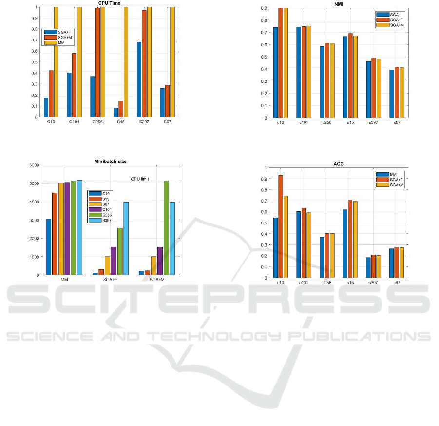
Figure 1: CPU time of SGA learners as a factor of batch
learner (MM). Lesser time is better.
Figure 2: Batch size capped at 5000 random samples for
MM. Least minibatch size for SGAs to achieve similar ACC
to MM. Smaller size reduces computational time.
dataset) and SGA (minibatch of 100 and 300 respec-
tively) for 30 iterations each. We observed that all
SGAs outperforms MM on all 5 evaluation criteria for
both datasets in terms of NMI and Accuracy, closer
to ground truth model selection, faster to compute as
a direct consequence of smaller sample size per it-
eration. The clustering performance (ACC & NMI)
of the proposed methods are indeed on-par or better
than MM. Also, it is evident that using SGAs allows it
to significantly reduce the computation time as com-
pared to its batch counterpart MM. This finding is ac-
tually consistent throughout all the datasets.
Next, we look at dataset #2 (Caltech101), #5
(MIT67) and #3 (Caltech256). These datasets are
slightly more challenging as they have 67-256 classes
and about 2-10 times the image size than earlier at
about 8K, 15K and 30K. We set the initial truncation
level to about twice the ground truth at 200, 100 and
500 respectively. For batch learners such as MM or
VI, they cannot handle these kind of dataset as the en-
tire datset size is too large. Instead, we fix the batch
size at around 5K and take a random subset of the
entire dataset that do not change for each iteration.
Meaning there is a large portion of dataset that MM
will never see. This is where SGAs are handy as it
Figure 3: NMI for closed form (MM) vs SGA learners.
Larger NMI is better.
Figure 4: Accuracy for closed form (MM) vs SGA learners.
Larger ACC is better.
can skip and access the entire dataset when the num-
ber of iterations increases as compared to MM. We set
the minibatch size to 1515 (10 random samples per
class), 1005 (15 random samples per class) and 2560
(10 random samples per class) respectively. We can
see that after 30 iterations, SGAs outperforms MM
once again on all 5 criteria.
Lastly, we look at dataset #6 (SUN397). This
dataset is considered quite large at >0.1M images and
almost 400 class. Using 1000 classes for truncation
level, we see that MM is unable to learn as quickly
as SGAs after 30 iterations as the estimated model is
quite large at 838 compared to 570.5 for the SGA+F.
Also for SGAs, there are some minor improvements
for NMI and ACC as compared to MM. The compu-
tational time is also 30% faster for SGA+F.
6 COMPARISON WITH
LITERATURE
In this section, we are mainly comparing the cluster-
ing performance of our proposed method with results
reported by the state–of-the-arts methods.
Variational Inference of Dirichlet Process Mixture using Stochastic Gradient Ascent
39
Table 1: Datasets partitioned (Caltech, Scenes) for our ex-
periments.
Dataset Train Test
Caltech10 500 2544
Caltech101 3030 5647
Caltech256 7680 22,102
Scene15 750 3735
MIT67 3350 12,270
SUN397 39,700 69,054
Table 2: Model Selection.
Truth Trunc. MM SGA+F SGA+M
10 50 13.3 11.7 24
101 200 126.3 118.7 139.7
256 500 464.7 314.2 392.7
15 50 17.7 18 19
67 100 81.8 74.6 84.3
397 1000 838 570.5 577
6.1 Baselines
We conducted a literature search of recent Bayesian
nonparametrics citing the datasets we use. We first
discuss the baselines in Table 3 as follows: MMGM
(Chen et al., 2014), DDPM-L (Nguyen et al., 2017),
LDPO (Wang et al., 2017), DPmeans (Kulis and Jor-
dan, 2012), VB-DPM (Blei et al., 2006), MM-DPM
(Lim and Wang, 2018) and OnHGD(Fan et al., 2016).
We also implemented SVI (Hoffman et al., 2013) for
DPM.
6.2 Features
MMGM and DDPM-L are using the 128 dimensional
SIFT features. DPmeans, VB-DPM and MM-DPM
are using the 2048 dimensional sparse coding based
Fisher vector in (Liu et al., 2014). For LDPO, the au-
thors use the FC7 of Alexnet pretrained on Imagenet.
We did not cite the patch mining variant of LDPO as
it is mainly related to feature extraction rather than
BNP, hence it is not a direct comparison. For our im-
plementation of SVI, we use VGG16 pretrained on
ImageNet. For our proposed method, we use VGG16
pretrained on Place205 as the image feature extractor.
6.3 Truncation Level
The truncation level of MMGM and DDPM-L are not
given in (Nguyen et al., 2017). For LDPO, it is fixed
to the ground truth (Wang et al., 2017). For VB-DPM,
MM-DPM and SVI, the truncation setting are identi-
cal to this work. For DPmeans, we use ground truth
to initialize its parameter for convenience as reported
in (Lim and Wang, 2018).
6.4 Comparisons on Caltech10
We find that none of the baselines can outperform
the proposed method partly due to the discriminative
power that deep feature offers and the use of the pro-
posed stochastic optimization approach.
6.5 Comparisons on Scene15 & MIT67
In Table 6, LDPO-A-FC performs better than
SGA+Fisher on Accuracy for Scene15 but underper-
formed for NMI on MIT67. In fact, LDPO is only on
par with Kmeans for NMI on MIT67.
For DDPM-L and MMGM, there is a huge disad-
vantage on their results due to using handcrafted fea-
ture. However, from their extended results in (Nguyen
et al., 2017) we infer that the performance of DDPM-
L should be slightly better than DPM using MM when
the same deep feature is used.
In (Lim and Wang, 2018), MM-DPM is shown
to outperforms its VB-DPM counterpart on scene15.
Given that MM (of DPM) when assuming d = 0 is
almost similar to MM-DPM except without modeling
precision, the result of MM-DPM should be slightly
better than MM (of DPM) when using deep features.
6.6 Comparisons on Caltech101,
Caltech256 and SUN397
To the best of our knowledge, it is very rare to find
any recent BNP works addressing datasets beyond 67
classes for image datasets. The main reason is that it
is difficult to scale up BNP, which is one of the main
reason why we proposed the SGA learner over MM.
Although, the authors in (Fan et al., 2016) ap-
plied a BNP model to SUN397, they mainly use it for
learning a Bag-of-Words representation (Csurka et al.,
2004). It appears they then use a supervised learner
such as Bayes’s decision rule for classification. For
SUN397, the Accuracy reported in (Fan et al., 2016)
for their online hierarchical Dirichlet process mix-
ture of generalized Dirichlet (onHGD) is 26.52% on
SUN397. It is somewhat comparable to our Accuracy
of 20.9% using SGA since we do not use hierarchi-
cal representation nor generalized Dirichlet mixture.
The authors of (Fan et al., 2016) also reported an Ac-
curacy of 67.34% for SUN16. Although this is not a
direct comparison to Scene15 as the classes in SUN16
are different, it provides some insight on our method.
ICPRAM 2020 - 9th International Conference on Pattern Recognition Applications and Methods
40

Table 3: Recent Bayesian nonparametrics vs best proposed result on the object and scene categorization dataset. Evaluation
using NMI and Accuracy (in diamond bracket).
Caltech10 Scene15 MIT67 SUN397
MMGM (Chen et al., 2014) - 0.186 - -
-
DDPM-L (Nguyen et al., 2017) - 0.218 - -
-
DPmeans (Kulis and Jordan, 2012) 0.418 0.316
- -
VB-DPM (Blei et al., 2006) 0.446 0.317 - -
- -
MM-DPM (Lim and Wang, 2018) 0.387 0.321 - -
<39.14> <33.59>
Kmeans (Wang et al., 2017) - 0.659 0.386 -
<65.0> <35.6>
LDPO-A-FC (Wang et al., 2017) - 0.705 0.389 -
<73.1> <37.9>
OnHGD (Fan et al., 2016) - - - -
<67.34> <26.52>
SVI 0.810 0.670 0.413 0.489
<78.98> <63.56> <30.76> <23.93>
SGA+Fisher 0.898 0.70 0.53 0.60
<93.1> <70.3> <37.8> <31.9>
Our only concern is whether their result is attainable
using SIFT. Once again, we should point out that in
(Fan et al., 2016), the authors use OnHGD for learn-
ing a bag-of-words representation while our method
mainly learns the cluster mean of each class in Table
3.
7 CONCLUSION
Scalable algorithm of variational inference allows
Bayesian nonparametrics such as Dirichlet process
mixture to scale up to larger dataset at fractional
cost. In this paper, we target up to about 100K im-
ages and 400 object classes and high dimensional fea-
tures using VGG16 pretrained on ImageNet. How-
ever, the main problem is that most scalable Dirich-
let process mixture algorithms today still rely on the
closed form learning found in variational inference
from the past two decades. Stochastic gradient as-
cent is a modern approach to machine learning and
it is widely deployed in the training of deep neu-
ral networks. However, variational inference and
stochastic gradient ascent are mutually exclusive. In
this work, we propose using stochastic gradient as-
cent as a learner in variational inference. Unlike the
closed form learner in variational inference, stochas-
tic gradient ascent do not require closed form expres-
sion for learning the variational posterior expectata-
tions. However, stochastic gradient ascent alone is
not optimal for learning. It suffers from being a lo-
cal optimum approach and when applied to stochastic
dataset, it takes a long time to converge. Stochastic
optimization methods rely on decreasing step-size for
guaranteed convergence and better local search. Thus,
we explored using well known stochastic optimiza-
tion methods to improve the stochastic gradient ascent
learning of variational inference. Specifically, we ex-
plored Fisher information and the momentum method
to achieve a faster convergence. We compare our new
stochastic learner on the Dirichlet process Gaussian
mixture. We showed the performance gained in terms
of NMI, accuracy, model selection and computational
time on large scale datasets such as the MIT67, Cal-
tech101, Caltech256 and SUN397.
REFERENCES
Amari, S.-I. (1998). Natural gradient works efficiently in
learning. Neural computation, 10(2):251–276.
Bishop, C. M. (2006). Pattern recognition and machine
learning. springer.
Blei, D. M., Jordan, M. I., et al. (2006). Variational infer-
ence for dirichlet process mixtures. Bayesian analysis,
1(1):121–144.
Blei, D. M., Ng, A. Y., and Jordan, M. I. (2003). Latent
Variational Inference of Dirichlet Process Mixture using Stochastic Gradient Ascent
41

dirichlet allocation. the Journal of machine Learning
research, 3:993–1022.
Cai, D., He, X., and Han, J. (2005). Document clustering
using locality preserving indexing. IEEE Transactions
on Knowledge and Data Engineering, 17(12):1624–
1637.
Chen, C., Zhu, J., and Zhang, X. (2014). Robust bayesian
max-margin clustering. In Advances in Neural Infor-
mation Processing Systems, pages 532–540.
Csurka, G., Dance, C., Fan, L., Willamowski, J., and Bray,
C. (2004). Visual categorization with bags of key-
points. In Workshop on statistical learning in com-
puter vision, ECCV, volume 1, pages 1–2. Prague.
Fan, W., Bouguila, N., Du, J.-X., and Liu, X. (2018). Ax-
ially symmetric data clustering through dirichlet pro-
cess mixture models of watson distributions. IEEE
transactions on neural networks and learning systems,
30(6):1683–1694.
Fan, W., Sallay, H., and Bouguila, N. (2016). Online
learning of hierarchical pitman–yor process mixture
of generalized dirichlet distributions with feature se-
lection. IEEE transactions on neural networks and
learning systems, 28(9):2048–2061.
Goodfellow, I., Pouget-Abadie, J., Mirza, M., Xu, B.,
Warde-Farley, D., Ozair, S., Courville, A., and Ben-
gio, Y. (2014). Generative adversarial nets. In
Advances in neural information processing systems,
pages 2672–2680.
He, K., Zhang, X., Ren, S., and Sun, J. (2016). Deep resid-
ual learning for image recognition. In Proceedings of
the IEEE Conference on Computer Vision and Pattern
Recognition, pages 770–778.
Hoffman, M. D., Blei, D. M., Wang, C., and Paisley, J. W.
(2013). Stochastic variational inference. Journal of
Machine Learning Research, 14(1):1303–1347.
Honkela, A., Raiko, T., Kuusela, M., Tornio, M., and
Karhunen, J. (2010). Approximate riemannian con-
jugate gradient learning for fixed-form variational
bayes. Journal of Machine Learning Research,
11(Nov):3235–3268.
Honkela, A., Tornio, M., Raiko, T., and Karhunen, J.
(2007). Natural conjugate gradient in variational in-
ference. In International Conference on Neural Infor-
mation Processing, pages 305–314. Springer.
Kingma, D. P. and Welling, M. (2014). Stochastic gradi-
ent vb and the variational auto-encoder. In Second In-
ternational Conference on Learning Representations,
ICLR.
Krizhevsky, A., Sutskever, I., and Hinton, G. E. (2012). Im-
agenet classification with deep convolutional neural
networks. In Advances in neural information process-
ing systems, pages 1097–1105.
Kulis, B. and Jordan, M. I. (2012). Revisiting k-means:
New algorithms via bayesian nonparametrics. In Pro-
ceedings of the 29th International Conference on Ma-
chine Learning (ICML-12), pages 513–520.
Kurihara, K. and Welling, M. (2009). Bayesian k-means as
a maximization-expectation algorithm. Neural com-
putation, 21(4):1145–1172.
Lim, K.-L. and Wang, H. (2018). Fast approximation of
variational bayes dirichlet process mixture using the
maximization–maximization algorithm. International
Journal of Approximate Reasoning, 93:153–177.
Liu, L., Shen, C., Wang, L., van den Hengel, A., and Wang,
C. (2014). Encoding high dimensional local features
by sparse coding based fisher vectors. In Advances in
Neural Information Processing Systems, pages 1143–
1151.
Mandt, S., Hoffman, M. D., and Blei, D. M. (2017).
Stochastic gradient descent as approximate bayesian
inference. The Journal of Machine Learning Re-
search, 18(1):4873–4907.
Neal, R. M. and Hinton, G. E. (1998). A view of the em
algorithm that justifies incremental, sparse, and other
variants. In Learning in graphical models, pages 355–
368. Springer.
Nguyen, V., Phung, D., Le, T., and Bui, H. (2017). Dis-
criminative bayesian nonparametric clustering. In IJ-
CAI 2017: Proceedings of the 26th International Joint
Conference on Artificial Intelligence, pages 2550–
2556. AAAI Press.
Paisley, J., Blei, D. M., and Jordan, M. I. (2012). Variational
bayesian inference with stochastic search. In Proceed-
ings of the 29th International Coference on Interna-
tional Conference on Machine Learning, pages 1363–
1370. Omnipress.
Paisley, J., Wang, C., Blei, D. M., and Jordan, M. I. (2015).
Nested hierarchical dirichlet processes. IEEE trans-
actions on pattern analysis and machine intelligence,
37(2):256–270.
Ranganath, R., Gerrish, S., and Blei, D. (2014). Black box
variational inference. In Artificial Intelligence and
Statistics, pages 814–822.
Rezende, D. J. and Mohamed, S. (2015). Variational in-
ference with normalizing flows. In Proceedings of
the 32nd International Conference on International
Conference on Machine Learning-Volume 37, pages
1530–1538. JMLR. org.
Robbins, H. and Monro, S. (1985). A stochastic approxi-
mation method. In Herbert Robbins Selected Papers,
pages 102–109. Springer.
Sethuraman, J. (1994). A constructive definition of dirichlet
priors. Statistica sinica, pages 639–650.
Titterington, D. M. (2011). The em algorithm, variational
approximations and expectation propagation for mix-
tures. Mixtures: Estimation and Applications, 896.
Wang, X., Lu, L., Shin, H.-C., Kim, L., Bagheri, M.,
Nogues, I., Yao, J., and Summers, R. M. (2017). Un-
supervised joint mining of deep features and image
labels for large-scale radiology image categorization
and scene recognition. In Applications of Computer
Vision (WACV), 2017 IEEE Winter Conference on,
pages 998–1007. IEEE.
Welling, M. and Teh, Y. W. (2011). Bayesian learning via
stochastic gradient langevin dynamics. In Proceed-
ings of the 28th International Conference on Machine
Learning (ICML-11), pages 681–688.
ICPRAM 2020 - 9th International Conference on Pattern Recognition Applications and Methods
42
