
Joint Optimization of Dynamic Lot-sizing and Condition-based
Maintenance
Alp Darendeliler
1
, Dieter Claeys
1,3
, Abdelhakim Khatab
2
and El-Houssaine Aghezzaf
1,3
1
Department of Industrial Engineering and Product Design, Ghent University, Gent, Belgium
2
Laboratory of Industrial Engineering, Production and Maintenance, Lorraine University, Metz, France
3
Industrial Systems Engineering (ISyE), Flanders Make, Belgium
www.FlandersMake.be
Keywords: Condition-based Maintenance, Lot-sizing, Stochastic Dynamic Programming.
Abstract: This study investigates the dynamic lot-sizing problem integrated with Condition-based maintenance (CBM)
for a stochastically deteriorating production system. The main difference of this work and the previous
literature on the joint optimization of lot-sizing and CBM is the relaxation of the constant demand assumption.
In addition, the influence of the lot-size quantity on the evolution of the equipment degradation is considered.
To optimally integrate production and maintenance, a stochastic dynamic programming model is developed
that optimizes the total expected production and maintenance cost including production setup cost, inventory
holding cost, lost sales cost, preventive maintenance cost and corrective maintenance cost. The algorithm is
run on a set of instances and the results show that the joint optimization model provides considerable cost
savings compared to the separate optimization of lot-sizing and CBM.
1 INTRODUCTION
Preventive maintenance operations aim to keep the
equipment in operating condition and reduce the
chance of having failures. Under Condition-based
maintenance, they are performed based on the current
condition of the equipment obtained through
Condition monitoring (Jardine, 2005). It can
significantly reduce maintenance cost by eliminating
unnecessary scheduled preventive maintenance
operations (Jardine, 2005).
To not interrupt the production, preventive
maintenance actions should be conducted in
accordance with the production plan in deteriorating
production systems. Since machine deterioration
depends on the amount of usage, the production
planning decisions directly affect degradation of the
systems. Thus, degradation of the equipment should
be considered in determining production amounts. To
address this issue, integrated optimization models of
Economic Production Quantity (EPQ) and CBM were
developed under the assumption of constant demand
rate. Producing same quantity in each lot, leads to the
same expected degradation path in those systems.
Therefore, applying a static maintenance policy is
convenient.
In a dynamic lot-sizing problem, however,
production time and thus equipment usage within
each period may differ, leading to different
degradation paths. Using a static preventive
maintenance threshold may not be optimal in this
case. Therefore, for each period, a dynamic
maintenance policy that considers future degradation
paths with respect to different production quantities
should be utilized.
This paper proposes a model to consider the
current equipment condition and the evolution of the
degradation with respect to production quantity in
making production and maintenance decisions.
Demanded quantities of the remaining periods,
current condition of the equipment, and inventory
level are the states that determine the production and
maintenance policies for each period. The main
difference of our work with the previous papers is the
adaption of CBM to the multi-period lot-sizing
problem under dynamic demand. In addition, in our
work, the influence of the quantity of the lot-size on
the degradation level is taken into account in
determining production decisions which has not been
considered in this problem setting. We construct a
stochastic dynamic programming model to minimize
production setup cost, inventory holding cost, lost
Darendeliler, A., Claeys, D., Khatab, A. and Aghezzaf, E.
Joint Optimization of Dynamic Lot-sizing and Condition-based Maintenance.
DOI: 10.5220/0008941601510158
In Proceedings of the 9th International Conference on Operations Research and Enterprise Systems (ICORES 2020), pages 151-158
ISBN: 978-989-758-396-4; ISSN: 2184-4372
Copyright
c
2022 by SCITEPRESS – Science and Technology Publications, Lda. All rights reserved
151

sales cost, preventive maintenance and corrective
maintenance costs over finite and infinite horizons.
2 LITERATURE REVIEW
The joint optimization of lot-sizing and maintenance
problem has been extensively studied under
breakdown, time-based and age-based maintenance.
Groenevelt et. al (1992) investigates the effect of
machine breakdowns and corrective maintenance on
the optimal production lot-sizes. They examine the
effect of the failure rate on the optimal lot-size
quantity. Ben-Daya and Makhdoum (1998) consider
an integrated production and quality model for
different inspection policies and they model the
deterioration process using hazard rate function. They
investigate the impact of different preventive
maintenance policies on the EPQ. Ben-Daya (2002)
proposes an integrated optimization model for lot-
sizing and imperfect preventive maintenance which
adopts age-based maintenance policy. El-Ferik
(2008) considers economic production lot-sizing for
an unreliable machine under constant production and
demand rates. Preventive maintenance actions are
carried out when the age of the system reaches a
predetermined level. After each preventive
maintenance, the system becomes as good as new
with a high failure rate. Thus, the system is replaced
after a certain amount of production cycles are
completed. Jafari and Makis (2015) study optimal lot-
sizing and preventive maintenance policy where the
deterioration is modeled by a proportion hazards
model which considers information gathered from
condition monitoring and age of the system. They
model and solve the problem as a semi-Markov
decision process.
Stochastic dynamic programing models are also
developed to optimize production and maintenance
costs. Boukas and Liu (2001) propose a stochastic
dynamic programming model to minimize
maintenance and inventory holding costs by
optimizing production and maintenance rates. Iravani
and Duenyas (2002) consider an integrated
maintenance and production control for a single item
single machine production system with increasing
failure rate. The demand is distributed as a stationary
Poisson process. They formulate the problem as a
Markov Decision Process (MDP) where the states are
degradation and inventory levels, and the actions are
producing, idling and maintenance at each decision
epoch. Sloan (2004) and Xiang et al. (2014) consider
integrated production and maintenance planning
subject to random production yield that changes with
respect to the condition of the equipment. The
maintenance and production planning decisions are
made according to the degradation status of the
equipment and yield. However, the influence of the
production amount on the machine deterioration is
not taken into account.
The joint optimization problem of Economic
Production Quantity (EPQ) and CBM is studied under
the assumption of constant production and demand
rates. Peng and Van Houtum (2016) propose a joint
optimization model of EPQ and CBM in which
degradation is modeled as Gamma Process. Khatab
et al. (2017) develop an integrated optimization
model for production quality and CBM. The
preventive maintenance threshold and inspection
interval are the decision variables. However, the lot-
size is not optimized. Cheng et. al (2017) propose a
joint optimization model for production lot-sizing and
CBM for a multi-component production system.
Degradation of the components are modeled by
Gamma process. They use Birnbaum importance
measure to determine the preventive maintenance
threshold of the components. Monte Carlo simulation
technique is used to calculate the costs and genetic
algorithm is utilized to find the optimal lot-size and
preventive maintenance threshold.
Maintenance scheduling has been incorporated in
the multi-item lot-sizing problems in which cyclic or
non-cyclic maintenance actions are performed.
Aghezzaf et. al (2007) propose an integrated
production and preventive maintenance model for a
capacitated multi-item production system in which
the overall capacity of the system is reduced when a
preventive or corrective maintenance is conducted.
They consider capacity reduction of the production in
case of failure or preventive maintenance. Preventive
maintenance actions are carried out at periodic time
points. Shamsaei and Van Vyve (2017) also develop
an integrated model for multi-item lot-sizing and
maintenance under time-varying demand.
Additionally, they adapt non-cyclic maintenance
schedules to their model which reduces the overall
costs. However, preventive maintenance actions are
performed without considering the health status of the
component.
3 SYSTEM DESCRIPTION
We consider a production system in which the
degradation of the machine is monitored
continuously. Its level
increases with respect to
the length of the production run-time. When the
machine fails during the period, and thus the
ICORES 2020 - 9th International Conference on Operations Research and Enterprise Systems
152
degradation having reached the “failure level” , the
production stops, and corrective maintenance is
conducted. Note that in case of a failure during a
period,
the remaining units of production cannot be
produced, although it was planned. To reduce the
possibility of the failures, preventive maintenance
actions are performed while the equipment is still in
working condition.
Nomenclature
degradation level with respect to
time
degradation level at the beginning of
period
state of Markov chain right after the
production of
unit within a
period
inventory level at the end of period
first passage time to failure from
state
production lot size in period
,,
optimal production lot size in period
n for states and
indicator variable taking value 1 if
there is production in period
indicator variable taking value 1 if
there is enough inventory and
production to cover the demand up
to the failure
production rate per unit time
constant demand rate per unit time
during period
total demand in period
fixed time length of a period
finite number of periods
inventory holding cost per unit of
time
lost sales cost per unit
production setup cost per lot
predictive maintenance cost
corrective maintenance cost
,
inventory holding as a function of
and
in case of no failure
,
inventory holding as a function of
and
in case of failure
,
lost sales cost as a function of
and
,
total minimum expected cost from
time to the end of the planning
horizon
discount factor
At the beginning of each period with a fixed
length , a preventive maintenance decision is made
and quantity of the production lot size
is
determined according to the current degradation level
, the ending inventory of the previous period
,
and known demand values of the remaining periods.
The production rate is constant so the maximum
amount of production in a period is limited to . If
there is no failure within the production lot and thus
the production plan is met for that period, there are
two cases: (1) no maintenance is carried out so the
starting degradation state of the next period is equal
to the ending degradation state of the current period;
(2) preventive maintenance is carried out at the
beginning of the next period; in this case, starting
degradation state of the next period becomes as good
as new. Because maintenance duration is assumed to
be negligible, carrying out maintenance at the end of
the production time within a period or at the
beginning of the next period does not make a
difference for the model. To be comprehensible, it is
assumed that maintenance actions are conducted at
the beginning of the periods.
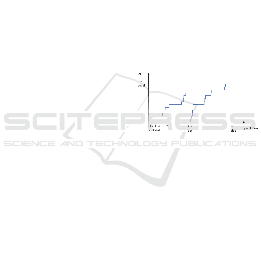
Figure 1: Sample degradation path with respect to
production time.
Figure 1 shows an example of a sample
degradation path starting from as good as new state
with respect to the production time where preventive
maintenance is carried out right after the completion
of
item’s production. The health status of the
machine becomes as good as new after that point. A
failure occurs after the production of the
item so
corrective maintenance is performed starting from
this point. The corresponding graph of the inventory
level with respect to the total time including the
production and idle times are illustrated in Figure 2.
During the idle times when the production capacity is
not fully utilized, the degradation remains in the same
level.
In the example shown, corrective maintenance is
conducted in the
period, starting right after the
production of the
item. Since there is not enough
inventory to cover the demand at the
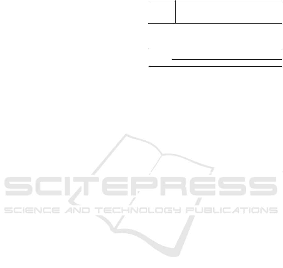
period, lost
sales occur. Figure 3 shows the case where sufficient
amount of inventory is accumulated up to the failure,
so no lost sales occurs. In the example shown in
Figures 1 and Figure 2, up to the
period, total
Joint Optimization of Dynamic Lot-sizing and Condition-based Maintenance
153
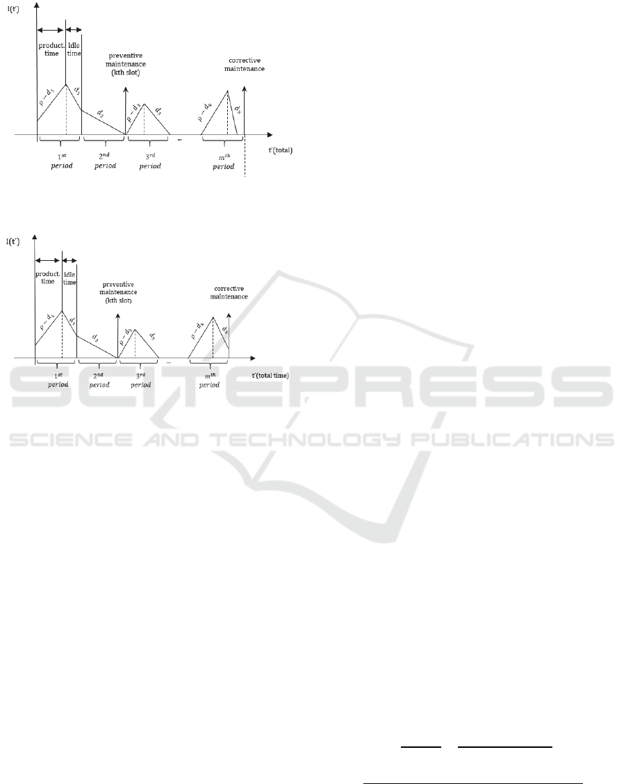
amount of production is equal to
∑
∑
; which is less than the planned production
amount due to the failure.
Figure 2: Inventory level with respect to total time
including production and idle times.
Figure 3: Inventory level with respect to total time
including production and idle times.
4 MODEL FORMULATION
The evolution of the degradation during production
time is modeled as a discrete-time stochastic process.
The
epoch corresponds to the planned completion
epoch of the
unit. As a result, the time in between
two planned production epochs within the same
period equals 1/, with the production rate. The
degradation level at epoch is denoted by
. Within
a period, the process
,0,1,…
, behaves as an
absorbing Markov chain with state space
0,1,…,
,
absorbing state , and transition probabilities
of
degradation level transitioning to state at the next
epoch if the degradation level is equal to at the
current epoch. It is given by
|
,
(1)
As degradation cannot decrease during a period,
0 if . denotes the matrix of one-step
transition probabilities
. It can be expressed as
1
,
(2)
where is the probability transition matrix of the
transient states of (first row and columns of),
and is the column vector showing the probabilities
from each state to the failure state (first
rows of the last column of ).
The -step transition probability of the Markov
chain from state to corresponds to the probability
that the degradation is at level right after the
production of the
item within the same period. It
is given by
|
.
(3)
Since is the absorbing state of the Markov chain,
|
1
∀∈
1,2,…
.
(4)
is equal to the entry at the
row and
column of the transition probability matrix
.
If
items are planned to be produced in period
and the degradation level at the beginning of the
period is , then
is the probability that state
will be observed at the end of the production run. If
a failure occurs right after the production of the
unit (
, before the production of the
unit, the production is stopped. The first passage time
, from state to the failure state , has the phase-
type distribution (
,), that is
.
.,
(5)
1
.
.,
(6)
where
is the
unit vector. Note that
takes
values in terms of units of quantity produced up to the
failure.
In case of no failure, the inventory holding cost in
period, where the production lot-size and initial
inventory level are
and
, is given by
,
⁄
2
⁄
⁄
2
⁄
,
(7)
ICORES 2020 - 9th International Conference on Operations Research and Enterprise Systems
154

where
is the inventory holding cost per item per
unit time,
is the total demand of the period and
is the demand rate during period that is equal to
⁄
. The equation is obtained by the integration of
the inventory level with respect to total time as
illustrated in Figure 2; it is equal to the area under the
curve within a period .
At the beginning of a period, if the degradation is
observed to be in state , inventory level is
and a
failure occurs during production, then the inventory
holding cost is expressed as
,
1
2
2
2
2
,
(8)
and the indicator variable is given by
1
0
0.
(9)
In case of a failure, two cases can occur: (1) the
total demand is covered (
; (2)
demand is not met and lost sales cost is incurred
(
). The equations for calculating the
area under the inventory level differs in these cases so
indicator variable
is used. In
case of a failure, the lost sales cost is given by
,
max0,
,
(10)
where the initial degradation level is and the lost
sales cost per item is
as in the
production lot
(Figure 2). The dynamic programming equation in
period for states and
is expressed as
,
,
,
∑
,
,
,
,
,
0,
,
,
,
,
,
,
0,
.
(11)
denotes the production capacity in terms of units,
that is equal to . The feasible production lot-size
in state
,
, must be in
max
,0,min,
∑
.
If a failure occurs in the previous period, then the
initial degradation state at the beginning of the period
is , and the dynamic programming equation is
given by,
,
,
,
∑
,
,
,
,
,
0,
.
(12)
In this case, corrective maintenance is done and its
cost
is incurred. In the dynamic programming
equations, the indicator variable
takes 1 if
there is production in period . It can be expressed as
1
0
0.
(13)
Joint Optimization of Dynamic Lot-sizing and Condition-based Maintenance
155
,
is the total minimum expected cost
between and and 0
min1
∑
,
∑
). The ending value
,
, is 0 for all
and
and the final
inventory level
0. To find the optimal production
and maintenance policy, enumeration is done over all
feasible values of
in case of preventive
maintenance and no preventive maintenance. Thus, the
optimal policy for each period , degradation level
and initial inventory level
is found.
0,
is the total minimum expected cost value for the
whole horizon where the initial degradation level
is
0 and the initial inventory level is
. is the
production capacity that is equal to the . The
discount factor is used for the infinite horizon case;
it is taken as 1 for finite horizon problem.
5 NUMERIC STUDY
In this example, the degradation is modelled as a
discrete-time Markov chain having8 states. State0 is
the as good as new state and state 7 is the failure state.
The mean time to failure from state 0 is 8.85 in terms
of units produced. The inventory holding cost per
item per unit time is
1, the production setup cost
is
150, the cost of the preventive maintenance is
500, the cost of the corrective maintenance is
1000and the cost of lost sales per item is
500. The problem is solved for changing demand
values (Table 1) which are randomly generated
integers in
0,10
for finite horizon 10. The
production rate and fixed time length of one period
are 2 and 10 respectively.
The optimal production and maintenance plan for
the periods between 6 and 10 are shown in Table 2
for the specified degradation and inventory states. For
the degradation state and the initial inventory level
in period ,
,,
shows the optimal
production quantity; optimal maintenance decision is
shown by either performing preventive maintenance
“P” or not “N”. Since preventive maintenance is
always carried out when degradation level is greater
than or equal to 3, same production quantities are
optimal as in thedegradation state 0. Infeasible states
are indicated by “-“. It can be seen from the Table 2
that if a preventive maintenance action is not carried
out in a period, then optimal production quantity is
non-decreasing with the degradation level for the
same inventory level . For instance, optimal
production lot sizes for period 8 and initial
inventory level 5 are:
0,5,8
1,
1,5,8
9,
2,5,8
9,
3,5,8
4.
Table 1: Demand values for each period.
Period 1 2 3 4 5 6 7 8 9 10
Demand 5 8 4 3 3 5 9 8 6 2
Table 2: Optimal production and maintenance policies for
each state and period.
Periodn
State 6 7 8 9 10
0,2,n 13,N 15,N 12,N 6,N 0,N
1,2,n 12,N 11,N 12,N 6,N 0,N
2,2,n 8,N 10,N 7,N 6,N 0,N
3,2,n
6,N 15,P 12,P 4,N 0,N
0,3,n 13,N 14,N 13,N 5,N ‐
1,3,n 12,N 11,N 11,N 5,N ‐
2,3,n 11,N 10,N 11,N 5,N ‐
3,3,n 6,N 14,P 5,N 5,N ‐
0,4,n 12,N 13,N 12,N 4,N ‐
1,4,n 11,N 13,N 10,N 4,N ‐
2,4,n
10,N 9,N 10,N 4,N ‐
3,4,n 5,N 6,N 4,N 4,N ‐
0,5,n 0,N 12,N 11,N 3,N ‐
1,5,n 0,N 12,N 9,N 3,N ‐
2,5,n 9,N 8,N 9,N 3,N ‐
3,5,n 5,N 6,N 4,N 3,N ‐
5.1 Sensitivity Analysis and
Performance Evaluation
In this part, the objective function values of the joint
optimization model are compared with the separate
optimization model. In the separate optimization
model, first, the production plan is found by
minimizing the production costs without considering
maintenance. Then, optimal preventive maintenance
decision for each state
,
is found; the
production quantities are known from the first stage.
The model is tested for different levels of the
production setup cost
, the preventive maintenance
cost
and the inventory holding cost
. The value
of each parameter is changed while other parameters
are kept
at their initial values:
150,
1,
500,
250,
1000,10 and the total
demand of each period is generated as a random
integer in
0,10
for each instance. The beginning
and the ending inventory levels,
and
are both
chosen as zero, and the initial degradation level
is
0.
The cost savings are calculated for five
independently generated demand values, and they are
shown in the following tables. Cost savings
percentages are calculated by
ICORES 2020 - 9th International Conference on Operations Research and Enterprise Systems
156

,
,
100
,
,
(14)
where
,
is the total expected minimum cost
of separate optimization model.
As shown in Table 3, the cost saving percentages
of the joint optimization model are mostly at the
highest level for the production setup cost
50
and it decreases with the increasing values of
for
each instance. When the setup cost is high, the joint
optimization model proposes higher production lot
sizes which leads to higher risks of having failure.
Thus, the percentage of cost savings are low in this
case. The optimal production lot-sizes are relatively
low when the setup cost is lower, so the machine
degrades less in each lot. Therefore, the possibility of
having failures and lost sales are lower that leads to
higher cost savings.
Table 3: Percentage of Saving (SP) for different values of
setup cost c
.
c
Instance 50 150 400
1 15.59% 16.94% 5.57%
2 14.45% 10.88% 5.94%
3 7.67% 5.93% 4.32%
4 19.04% 12.8% 6.05%
5 24.44% 17.97% 10.89%
Average 16.24% 12.90% 6.53%
For higher levels of preventive maintenance cost
values, the amount of the percentage of savings are
observed to be less for each instance since changes in
the production plans are less effective for reducing
the overall costs (Table 4).
Table 4: Percentage of Saving (SP) for different values of
preventive maintenance cost
.
c
Instance 250 500 750
1 18.12% 8.21% 5.80%
2 16.72% 5.66% 3.25%
3 7.62% 4.17% 5.79%
4 13.96% 5.34% 2.99%
5 15.06% 5.86% 3.59%
Average 14.29% 5.84% 4.28%
Table 5 shows the cost savings of the separate and
joint optimization models for three different levels of
the inventory holding cost. When
is low, optimal
lot-sizes tend to be higher in the separate optimization
model minimizing only production setup and
inventory holding costs. Because keeping more
inventory and having a smaller number of production
runs minimize the total production costs, separate
optimization model proposes higher quantities of
production for low inventory holding cost values;
therefore, there is a higher risk of having corrective
maintenance and lost sales.
Table 5: Percentage of Saving (SP) for different values of
inventory holding cost
.
c
Instance 0.5 1 2
1 12.95% 9.30% 9.88%
2 15.47% 7.39% 5.52%
3 12.09% 5.57% 4.12%
4 15.73% 14.63% 9.36%
5 10.15% 8.50% 8.89%
Average 13.28% 9.08% 7.55%
6 CONCLUSIONS
In this study, joint optimization of lot-sizing and
CBM is studied under time-varying demand for a
deteriorating production system. The effect of the lot-
size on the machine degradation is considered. A
stochastic dynamic programming model is
constructed to find the optimal policy to minimize
production setup cost, inventory holding cost, lost
sales cost, preventive maintenance and corrective
maintenance costs for finite horizon. The proposed
optimal policy is dynamic; it gives the optimal
production and maintenance decisions for each
degradation state, inventory level and period so it
minimizes overall costs from the current period to the
end of the planning horizon.
Numeric study is conducted to present the optimal
results of the model. Total costs of the joint and
separate optimization models are calculated, and the
cost savings are shown for the different levels of the
cost parameters. The parameters in the numeric
example are randomly selected to test the model. To
test the applicability of the proposed model, it could
be solved for the cases motivated by practice.
For future research, uncertain demand could be
considered for the integrated optimization of lot-
sizing and CBM. Adapting the imperfect maintenance
to our model, which relaxes the assumption that the
Joint Optimization of Dynamic Lot-sizing and Condition-based Maintenance
157

machine is as good as new after each maintenance
action, will be investigated. Multi-item production
systems may be studied for the future research as
well.
REFERENCES
Aghezzaf E. H., Jamali M., & Ait-Kadi D. (2007). An
integrated production and preventive maintenance
planning model. European Journal of Operational
Research, 181 (2), 679–685.
Ben-Daya M., Makhdoum M (1998). Integrated production
and quality model under various preventive
maintenance policies. Journal of the Operational
Research Society, 49(8), 840-853.
Ben-Daya, M. (2002). The economic production lot-sizing
problem with imperfect production processes and
imperfect maintenance. International Journal of
Production Economics, 76 (3), 257–264.
Boukas E., & Liu Z. (2001). Production and maintenance
control for manufacturing systems. IEEE Transactions
on Automatic Control, 46 (9), 1455–1460.
Cheng Q. C., Zhou B. H., Li L. Joint optimization of lot
sizing and condition-based maintenance for multi-
component production systems, Computers &
Industrial Engineering, 110, 538-549.
El Ferik S. (2008). Economic Production lot-sizing for an
unreliable machine under imperfect age-based
maintenance policy. European Journal of Operational
Research 186(1):150–163.
Groenevelt H., Pintelon L., & Seidmann A. (1992).
Production lot sizing with ma chine breakdowns.
Management Science, 38, 104–123.
Iravani S., & Duenyas I. (2002). Integrated maintenance
and production control of a deteriorating production
system. IIE Transactions, 34 (5), 423–435.
Jardine, A., Lin, D., & Banjevic, D. (2006). A review on
machinery diagnostics and prognostics implementing
condition-based maintenance. Mechanical Systems and
Signal Processing, 20, 1483–1510.
Khatab A., Diallo C., Aghezzaf E. & Venkatadri U. (2018).
Integrated production quality and condition-based
maintenance for a stochastically deteriorating
manufacturing system. International Journal
Production Research, 57(8). p.2480-2497.
Peng H., G.-J. Van Houtum. 2016. Joint Optimization of
Condition-based Maintenance and Production Lot-
sizing. European Journal of Operational Research 253:
94–107.
Shamsaei F., Van Vyve M. (2017), Solving integrated
production and condition-based maintenance planning
problems by MIP modeling. Flexible Services and
Manufacturing Journal, 29:184-202.
Sloan, T. W. 2004. “A Periodic Review Production and
Maintenance Model with Random Demand,
Deteriorating Equipment, and Binomial Yield.”
Journal of the Operational Research Society 55 (6):
647–656.
Xiang Y, Cassady CR, Jin T, Zhang CW (2014). Joint
production and maintenance planning with machine
deterioration and random yield. International Journal
Production Research, 52(6):1644–1657.
ICORES 2020 - 9th International Conference on Operations Research and Enterprise Systems
158
