Self-Training using Selection Network for Semi-supervised Learning
Jisoo Jeong
∗ a
, Seungeui Lee
∗ b
and Nojun Kwak
† c
Seoul National University, Seoul, South Korea
Keywords:
Semi-supervised Learning.
Abstract:
Semi-supervised learning (SSL) is a study that efficiently exploits a large amount of unlabeled data to improve
performance in conditions of limited labeled data. Most of the conventional SSL methods assume that the
classes of unlabeled data are included in the set of classes of labeled data. In addition, these methods do not
sort out useless unlabeled samples and use all the unlabeled data for learning, which is not suitable for realistic
situations. In this paper, we propose an SSL method called selective self-training (SST), which selectively
decides whether to include each unlabeled sample in the training process. It is designed to be applied to
a more real situation where classes of unlabeled data are different from the ones of the labeled data. For the
conventional SSL problems which deal with data where both the labeled and unlabeled samples share the same
class categories, the proposed method not only performs comparable to other conventional SSL algorithms but
also can be combined with other SSL algorithms. While the conventional methods cannot be applied to the
new SSL problems, our method does not show any performance degradation even if the classes of unlabeled
data are different from those of the labeled data.
1 INTRODUCTION
Recently, machine learning has achieved a lot of suc-
cess in various fields and well-refined datasets are
considered to be one of the most important factors
(Everingham et al., 2010; Krizhevsky et al., 2012;
Russakovsky et al., 2015). Since we cannot discover
the underlying real distribution of data, we need a
lot of samples to estimate it correctly (Nasrabadi,
2007). However, making a large dataset requires a
huge amount of time, cost and manpower (Chapelle
et al., 2009; Odena et al., 2018).
Semi-supervised learning (SSL) is a method re-
lieving the inefficiencies in data collection and an-
notation process, which lies between the supervised
learning and unsupervised learning in that both la-
beled and unlabeled data are used in the learning pro-
cess (Chapelle et al., 2009; Odena et al., 2018). It
can efficiently learn a model from fewer labeled data
using a large amount of unlabeled data (Zhu, 2006).
Accordingly, the significance of SSL has been stud-
ied extensively in the previous literatures (Zhu et al.,
a
https://orcid.org/0000-0003-1154-4532
b
https://orcid.org/0000-0003-3560-785X
c
https://orcid.org/0000-0002-1792-0327
* Equal contribution
†
Corresponding author.
2003; Rosenberg et al., 2005; Kingma et al., 2014;
Rasmus et al., 2015; Odena, 2016; Akhmedova et al.,
2017). These results suggest that SSL can be a useful
approach in cases where the amount of annotated data
is insufficient.
However, there is a recent research discussing
the limitations of conventional SSL methods (Odena
et al., 2018). They have pointed out that conventional
SSL algorithms are difficult to be applied to real ap-
plications. Especially, the conventional methods as-
sume that all the unlabeled data belong to one of the
classes of the training labeled data. Training with un-
labeled samples whose class distribution is signifi-
cantly different from that of the labeled data may de-
grade the performance of traditional SSL methods.
Furthermore, whenever a new set of data is available,
they should be trained from the scratch using all the
data including out-of-class
1
data.
In this paper, we focus on the classification task
and propose a deep neural network based approach
named as selective self-training (SST) to solve the
limitation mentioned above. To enable learning to se-
1
The term out-of-class is used to denote the situation
where the new dataset contains samples originated from
different classes than the classes of the old data. On the
other hand, the term in-class is used when the new data con-
tain only the samples belonging to the previously observed
classes.
Jeong, J., Lee, S. and Kwak, N.
Self-Training using Selection Network for Semi-supervised Learning.
DOI: 10.5220/0008940900230032
In Proceedings of the 9th International Conference on Pattern Recognition Applications and Methods (ICPRAM 2020), pages 23-32
ISBN: 978-989-758-397-1; ISSN: 2184-4313
Copyright
c
 2022 by SCITEPRESS – Science and Technology Publications, Lda. All rights reserved
23

lect unlabeled data, we propose a selection network,
which is based on the deep neural network, that de-
cides whether each sample is to be added or not. Dif-
ferent from (Wang et al., 2018), SST does not di-
rectly use the classification results for the data selec-
tion. Also, we adopt an ensemble approach which is
similar to the co-training method (Blum and Mitchell,
1998) that utilizes outputs of multiple classifiers to
iteratively build a new training dataset. In our case,
instead of using multiple classifiers, we apply a tem-
poral ensemble method to the selection network. For
each unlabeled instance, two consecutive outputs of
the selection network are compared to keep our train-
ing data clean.
In addition, we have found that the balance be-
tween the number of samples per class is quite impor-
tant for the performance of our network. We suggest
a simple heuristics to balance the number of selected
samples among the classes. By the proposed selection
method, reliable samples can be added to the training
set and uncertain samples including out-of-class data
can be excluded. The main contributions of the pro-
posed method can be summarized as follows:
• For the conventional SSL problems, the proposed
SST method not only performs comparable to
other conventional SSL algorithms but also can be
combined with other algorithms.
• For the new SSL problems, the proposed SST
does not show any performance degradation even
with the out-of-class data.
• SST requires few hyper-parameters and can be
easily implemented.
To prove the effectiveness of our proposed
method, first, we conduct experiments comparing the
classification errors of SST and several other state-of-
the-art SSL methods (Laine and Aila, 2016; Tarvainen
and Valpola, 2017; Luo et al., 2017; Miyato et al.,
2017) in conventional SSL settings. Second, we pro-
pose a new experimental setup to investigate whether
our method is more applicable to real-world situa-
tions. The experimental setup in (Odena et al., 2018)
samples classes among in-classes and out-classes. In
the experimental setting in this paper, we sample un-
labeled instances evenly in all classes. We evaluate
the performance of the proposed SST using three
public benchmark datasets: CIFAR-10, CIFAR-100
(Krizhevsky and Hinton, 2009), and SVHN (Netzer
et al., 2011).
2 BACKGROUND
In this section, we introduce the background of our
research. First, we introduce some methods of self-
training (McLachlan, 1975; Zhu, 2007; Zhu and
Goldberg, 2009) on which our work is based. Then we
describe consistency regularization-based algorithms
such as Π model and temporal ensembling (Laine and
Aila, 2016).
2.1 Self-training
Self-training method has long been used for semi-
supervised learning (McLachlan, 1975; Rosenberg
et al., 2005; Zhu, 2007; Zhu and Goldberg, 2009). It
is a resampling technique that repeatedly labels unla-
beled training samples based on the confidence scores
and retrains itself with the selected pseudo-annotated
data. This process can be formalized as follows. (i)
Training a model with labeled data. (ii) Predicting un-
labeled data with the learned model. (iii) Retraining
the model with labeled and selected pseudo-labeled
data. (iv) Repeating the last two steps.
However, most self-training methods assume that
the labeled and unlabeled data are generated from the
identical distribution. Therefore, in real-world sce-
narios, some instances with low likelihood accord-
ing to the distribution of the labeled data are likely
to be misclassified inevitably. Consequently, these er-
roneous samples significantly lead to worse results in
the next training step. To alleviate this problem, we
adopt the ensemble and balancing methods to select
reliable samples.
2.2 Consistency Regularization
Consistency regularization is one of the popular SSL
methods and has been referred to many recent re-
searches (Laine and Aila, 2016; Miyato et al., 2017;
Tarvainen and Valpola, 2017). Among them, Π model
and temporal ensembling are widely used (Laine and
Aila, 2016). They have defined new loss functions
for unlabeled data. The Π model outputs f (x) and
ˆ
f (x) for the same input x by perturbing the input
with different random noise and using dropout (Sri-
vastava et al., 2014), and then minimizes the dif-
ference (k f (x) −
ˆ
f (x)k
2
) between these output val-
ues. Temporal ensembling does not make different
predictions f (x) and
ˆ
f (x), but minimizes the differ-
ence (k f
t−1
(x) − f
t
(x)k
2
) between the outputs of two
consecutive iterations for computational efficiency. In
spite of the improvement in performance, they re-
quire lots of things to consider for training. These
methods have various hyper-parameters such as ‘ramp
ICPRAM 2020 - 9th International Conference on Pattern Recognition Applications and Methods
24

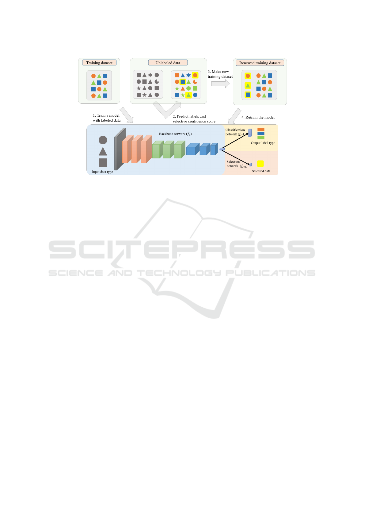
Figure 1: An overview of the proposed SST. Different shapes represent the input data with different underlying distribution,
and different colors (orange, blue, and green) are for different classes. In the initial training dataset, only three classes with
their corresponding distributions (#, 2, 4) exist and are used for initial training. Then the unlabeled data which include
unseen distribution (F, C) are inputted to the classification as well as the selection network. At the bottom right, unlabeled
samples with higher selection network output values than a certain threshold are denoted by yellow and selected to be included
in the training process for the next iteration, while the remaining are not used for training.
up’, ‘ramp down’, ‘unsupervised loss weight’ and
so on. In addition, customized settings for training
such as ZCA preprocessing and mean-only batch nor-
malization (Salimans and Kingma, 2016) are also
very important aspects for improving the performance
(Odena et al., 2018).
3 METHOD
In this section, we introduce our selective self-training
(SST) method. The proposed model consists of three
networks as shown in the bottom part of Figure 1.
The output of the backbone network is fed into two
sibling fully-connected layers —a classification net-
work f
cl
(·;θ
c
) and a selection network f
sel
(·;θ
s
),
where θ
c
and θ
s
are learnable parameters for each of
them. In this paper, we define the classification result
and the selection score as r
i
= f
cl
( f
n
(·;θ
n
);θ
c
) and
s
i
= f
sel
( f
n
(·;θ
n
);θ
s
), respectively, where f
n
(·;θ
n
)
denotes the backbone network with learnable param-
eters θ
n
. Note that we define r
i
as the resultant label
and it belongs to one of the class labels r
i
∈ Y =
{1, 2, ··· ,C}. As shown in Figure 1, the proposed SST
method can be represented in the following four steps.
First, SST trains the network using a set of the labeled
data L = {(x
i
, y
i
) | i = 1, ··· , L}, where x
i
and y
i
∈
{1, 2, ··· ,C} denote the data and the ground truth la-
bel respectively, which is a standard supervised learn-
ing method. The next step is to predict all the unla-
beled data U = {x
i
|i = L +1, ··· , N} and select a sub-
set of the unlabeled data {x
i
|i ∈ I
S
} whose data have
high selection scores with the current trained model,
where I
S
denotes a set of selected sample indices from
I
U
= {L + 1, ·· · , N}. Then, we annotate the selected
samples with the pseudo-categories ˆy
i
evaluated by
the f
cl
(·;θ
c
) and construct a new training dataset T
composed of L and U
S
= {(x
i
, ˆy
i
)|i ∈ I
S
}. After that,
we retrain the model with T and repeat this process it-
eratively. The overall process of the SST is described
in Algorithm 1 and the details of each of the four steps
will be described later.
3.1 Supervised Learning
The SST algorithm first trains a model with super-
vised learning. At this time, the entire model (all
three networks) is trained simultaneously. f
cl
(·;θ
c
)
is trained using the softmax function and the cross-
entropy loss as in the ordinary supervised classifica-
tion learning task. In case of f
sel
(·;θ
s
), the training la-
bels are motivated by discriminator of generative ad-
versarial networks (GAN) (Goodfellow et al., 2014;
Yoo et al., 2017). When x
i
with y
i
is fed into the net-
work, the target for f
sel
(·;θ
s
) is set as:
g
i
=
(
1, if r
i
= y
i
for i ∈ I
L
0, if r
i
6= y
i
for i ∈ I
L
(1)
where I
L
= {1, ··· , L} represents a set of labeled sam-
ple indices. f
sel
(·;θ
s
) is trained with the generated tar-
get g
i
. Especially, we use the sigmoid function for the
final activation and the binary cross-entropy loss to
Self-Training using Selection Network for Semi-supervised Learning
25

Algorithm 1: Training procedure of the proposed SST.
Require: x
i
, y
i
: training data and label
Require: L, U: labeled and unlabeled datasets
Require: I
U
: set of unlabeled sample indices
Require: f
n
(·;θ
n
), f
cl
(·;θ
c
), f
sel
(·;θ
s
): trainable SST
model
Require: α, ε, K, K
re
: hyper-parameters
1: randomly initialize θ
n
, θ
c
, θ
s
2: train f
n
(·;θ
n
), f
cl
(·;θ
c
), f
sel
(·;θ
s
) for K epochs
using L
3: repeat
4: initialize r
t
i
= −1, I
S
= ∅
5: for each i ∈ I
U
do
6: r
t−1
i
← r
t
i
, r
t
i
← f
cl
( f
n
(x
i
;θ
n
);θ
c
)
7: s
i
← f
sel
( f
n
(x
i
;θ
n
);θ
s
)
8: if r
t−1
i
6= r
t
i
then
9: z
i
← 0
10: end if
11: z
i
← αz
i
+ (1 − α)s
i
12: if z
i
> 1 − ε then
13: I
S
← I
S
∪ {i}
14: assign label for x
i
using r
i
15: end if
16: end for
17: update U
S
with data balancing
18: T ← L ∪ U
S
19: retrain f
n
(·;θ
n
), f
cl
(·;θ
c
), f
sel
(·;θ
s
) for K
re
epochs using T
20: until stopping criterion is true
train f
sel
(·;θ
s
). Therefore our f
sel
(·;θ
s
) does not uti-
lize the conventional softmax function because it pro-
duces a relative output and can induce a high value
even for an out-of-class sample. Instead, our f
sel
(·;θ
s
)
is designed to estimate an absolute confidence score
using the sigmoid activation function. More details
are provided in appendix. Consequently, our final loss
function is a sum of the classification loss L
cl
and the
selection loss L
sel
:
L
total
= L
cl
+ L
sel
. (2)
3.2 Prediction and Selection
After learning the model in a supervised manner, SST
takes all instances of U as input and predicts r
i
and
s
i
, for all i ∈ I
U
. We utilize r
i
and s
i
to annotate and
choose unlabeled samples, respectively. In the context
of self-training, removing erroneously annotated sam-
ples is one of the most important things for the new
training dataset. Thus, we adopt temporal co-training
and ensemble methods for the selection score in order
to keep our training set from contamination. First, let
Table 1: Ablation study with 5 runs on the CIFAR-10
dataset. ‘bal’ denotes the usage of data balancing scheme
during data addition as described in Sec. 3.3, ‘ens’ is for
the usage of previous selection scores as in the 11th line of
Algorithm 1.
method bal ens error
supervised learning 18.97 ± 0.37%
SST
x x 21.44 ± 4.05%
o x 14.43 ± 0.43%
o o 11.82 ± 0.40%
r
t
i
and r
t−1
i
be the classification results of the current
and the previous iterations respectively and we uti-
lize the temporal consistency of these values. If these
values are different, we set the ensemble score z
i
= 0
to reduce uncertainty in selecting unlabeled samples.
Second, inspired by (Laine and Aila, 2016), we also
utilize multiple previous network evaluations of un-
labeled instances by updating z
i
= αz
i
+ (1 − α)s
i
,
where α is a momentum weight for the moving aver-
age of ensemble scores. However, the aim of our en-
sembling approach is different from (Laine and Aila,
2016). They want to alleviate different predictions for
the same input, which are resulted from different aug-
mentation and noise to the input. However, our aim
differs from theirs in that we are interested in select-
ing reliable (pseudo-)labeled samples. After that, we
select unlabeled samples with high z
i
. It is very im-
portant to set an appropriate threshold because it de-
cides the quality of the added unlabeled samples for
the next training. If f
cl
(·;θ
c
) is trained well on the la-
beled data, the training accuracy would be very high.
Also, since f
sel
(·;θ
s
) is trained with g
i
generated from
r
i
and y
i
, s
i
will be close to 1.0. Therefore, we set the
threshold to 1− ε and control it by changing ε. In this
case, if z
i
exceeds 1 − ε, the pseudo-label of the unla-
beled sample ˆy
i
is set to r
i
.
3.3 New Training Dataset
When we construct T , we keep the number of sam-
ples of each class the same. The reason is that if
one class dominates the others, the classification per-
formance is degraded by the imbalanced distribution
(FernáNdez et al., 2013). We also empirically found
that naively creating a new training dataset fails to
yield good performance. In order to fairly transfer the
selected samples to the new training set, the amount
of migration in each class should not exceed the num-
ber of the class having the least selected samples.
We take arbitrary samples in every class as much as
the maximum number satisfying this condition. T is
composed of both L and U
S
. The number of selected
unlabeled samples is the same for all classes.
ICPRAM 2020 - 9th International Conference on Pattern Recognition Applications and Methods
26

Table 2: Classification error on CIFAR-10 (4k Labels), SVHN (1k Labels), and CIFAR-100 (10k Labels) with 5 runs using
in-class unlabeled data (* denotes that the test has been done by ourselves).
Method CIFAR-10 SVHN CIFAR-100
Supervised (sampled)* 18.97 ± 0.37% 13.45 ± 0.92% 40.24 ± 0.45%
Supervised (all)* 5.57 ± 0.07% 2.87 ± 0.06% 23.36 ± 0.27%
Mean Teacher (Tarvainen and Valpola, 2017) 12.31 ± 0.28% 3.95 ± 0.21% -
Π model (Laine and Aila, 2016) 12.36 ± 0.31% 4.82 ± 0.17% 39.19 ± 0.36%
TempEns (Laine and Aila, 2016) 12.16 ± 0.24% 4.42 ± 0.16% 38.65 ± 0.51%
TempEns + SNTG (Luo et al., 2017) 10.93 ± 0.14% 3.98 ± 0.21% 40.19 ± 0.51%*
VAT (Miyato et al., 2017) 11.36 ± 0.34% 5.42 ± 0.22% -
VAT + EntMin (Miyato et al., 2017) 10.55 ± 0.05% 3.86 ± 0.11% -
pseudo-label (Lee, 2013; Odena et al., 2018) 17.78 ± 0.57% 7.62 ± 0.29% -
Proposed method (SST)* 11.82 ± 0.40% 6.88 ± 0.59% 34.89 ± 0.75%
SST + TempEns + SNTG* 9.99 ± 0.31% 4.74 ± 0.19% 34.94 ± 0.54%
3.4 Re-training
After combining the labeled and selected pseudo-
labeled data, the model is retrained with the new
dataset for K
re
epochs. In this step, the label for the
f
sel
(·;θ
s
) is obtained by a process similar to Eq. (1).
Above steps (except for Section 3.1) are repeated for
M iterations until (near-) convergence.
4 EXPERIMENTS
To evaluate our proposed SST algorithm, we conduct
two types of experiments. First, we evaluate the pro-
posed SST algorithm for the conventional SSL prob-
lem where all unlabeled data are in-class. Then, SST
is evaluated with the new SSL problem where some
of the unlabeled data are out-of-class.
In the case of in-class data, gradually gathering
highly confident samples in U can help improve the
performance. On the other hand, in the case of out-
of-class data, a strict threshold is preferred to pre-
vent uncertain out-of-class data from being involved
in the new training set. Therefore, we have experi-
mented with decay mode that decreases the thresh-
old in log-scale and fixed mode that fixes the thresh-
old in the way described in Section 4.2. We have ex-
perimented our method with 100 iterations and deter-
mined ε by cross-validation in decay modes. In case
of fixed modes, ε is fixed and the number of iteration
is determined by cross-validation. The details about
the experimental setup is presented in appendix.
4.1 Conventional SSL Problems with
In-class Unlabeled Data
We experiment with three popular datasets which are
SVHN, CIFAR-10, and CIFAR-100 (Netzer et al.,
2011; Krizhevsky et al., 2014). The settings of labeled
versus unlabeled data separation for each dataset are
the same with (Laine and Aila, 2016; Miyato et al.,
2017; Tarvainen and Valpola, 2017). More details are
provided in appendix. Also, the network is the same
with (Laine and Aila, 2016).
4.1.1 Ablation Study
We have performed experiments on CIFAR-10 dataset
with the combination of two types of components. As
described in Table 1, these are whether to use data
balancing scheme described in Section 3.3 (balance),
whether to use selection score ensemble in the 11th
line of Algorithm 1 (ensemble). First, when SST does
not use all of these, the error 21.44% is higher than
that of the supervised learning which does not use
any unlabeled data. This is due to the problem of un-
balanced data mentioned in subsection 3.3. When the
data balance is used, the error is 14.43%, which is bet-
ter than the baseline 18.97%. Adding the ensemble
scheme results in 11.82% error. Therefore, we have
used only balance and ensemble schemes in the fol-
lowing experiments.
4.1.2 Experimental Results
Table 2 shows the experiment results of supervised
learning, conventional SSL algorithms and the pro-
posed SST on CIFAR-10, SVHN and CIFAR-100
datasets. Our baseline model with supervised learning
performs slightly better than what has been reported
in other papers (Laine and Aila, 2016; Tarvainen and
Valpola, 2017; Luo et al., 2017) because of our dif-
ferent settings such as Gaussian noise on inputs, opti-
mizer selection, the mean-only batch normalizations
and the learning rate parameters. For all the datasets,
we have also performed experiments with a model of
SST combined with the temporal ensembling (Tem-
Self-Training using Selection Network for Semi-supervised Learning
27

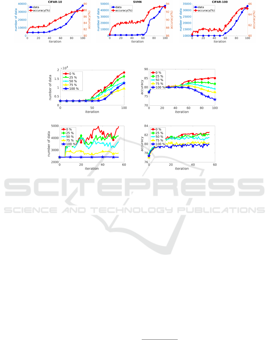
Figure 2: SST result on CIFAR-10, SVHN, and CIFAR-100 datasets with 5 runs. The x-axis is the iteration, the blue circle is
the average of the number of data used for training, and the red diamond is the average accuracy.
(a) (b)
(c) (d)
Figure 3: Result of new SSL problems on CIFAR-10 dataset with 5 runs. (a) number of data with iteration in decay mode
(b) accuracy with iteration in decay mode (c) number of data with iteration in fixed mode(d) accuracy with iteration in fixed
mode. % means the ratio of the number of non-animal classes in the unlabeled data.
pEns) and SNTG, labeled as SST+TempEns+SNTG.
For the model, the pseudo-labels of SST at the last it-
eration is considered as the true class label. Figure 2
shows the number of samples used in the training and
the corresponding accuracy on the test set for each
dataset.
CIFAR-10: The baseline network yields the test
error of 18.97% and 5.57% when trained with 4,000
(sampled) and 50,000 (all) labeled images respec-
tively. The test error of our SST method reaches
11.82% which is comparable to other algorithms
while SST+TempEns+SNTG model results 1.83%
better than the SST-only model.
SVHN: The baseline model for SVHN dataset is
trained with 1,000 labeled images and yields the test
error of 13.45%. Our proposed method has an er-
ror of 6.88% which is relatively higher than those
of other SSL algorithms. Performing better than SST,
SST+TempEns+SNTG reaches 4.74% of error which
is worse than that of TempEns+SNTG model. We
suspect two reasons for this. The first is that SVHN
dataset is not well balanced, and the second is that
SVHN is a relatively easy dataset, so it seems to be
easily added to the hard labels. With data balancing,
the SST is still worse than other algorithms. We think
this phenomenon owes to the use of hard labels in
SST where incorrectly estimated samples deteriorate
the performance.
CIFAR-100: While the baseline model results in
40.24% of error rate through supervised learning with
sampled data, our method performs with 34.89% of
error, enhancing the performance by 5.3%. We have
observed that the performance of TempEns+SNTG is
lower than TempEns, and when TempEns+SNTG is
added to SST, performance is degraded slightly. Al-
though TempEng+SNTG shows better performance
than TempEng without augmentation in (Luo et al.,
2017), its performance is worse than that of TempEng
with augmentation in our experiment. The reason for
this can be conjectured that the hyper-parameter in the
current temporal ensembling and SNTG may not have
been optimized
2
.
2
We have reproduced tempEns+SNTG model with a Py-
torch implementation, and have verified of its performance
on CIFAR-10 and SVHN akin to what is reported in (Luo
et al., 2017). However, for CIFAR-100 dataset, since the
experimental results without data augmentation are not re-
ported, we thus report our reproduced results.
ICPRAM 2020 - 9th International Conference on Pattern Recognition Applications and Methods
28

Table 3: Classification error for new SSL problems on CIFAR-10 and CIFAR-100 dataset with 5 runs. ’%’ means the ratio of
the number of non-animal classes.
dataset CIFAR-10 CIFAR-100
method SST(decay) SST(fixed) SST(decay) SST(fixed)
supervised 22.27 ± 0.47% 34.62 ± 1.14%
0% 14.99 ± 0.54% 17.84 ± 0.39% 28.01 ± 0.44% 32.16 ± 0.64%
25%
17.93 ± 0.33% 18.38 ± 0.52% 29.94 ± 0.45% 32.28 ± 0.58%
50% 20.91 ± 0.53% 19.04 ± 0.63% 31.78 ± 0.62% 32.60 ± 0.67%
75% 22.72 ± 0.42% 20.07 ± 0.98% 34.44 ± 0.85% 32.32 ± 0.52%
100% 26.78 ± 1.35% 20.24 ± 0.15% 37.17 ± 1.08% 32.62 ± 0.63%
4.2 New SSL Problems with
Out-of-class Unlabeled Data
We have experimented with the following settings
for real-world applications. The dataset is categorized
into six animal and four non-animal classes as simi-
larly done in (Odena et al., 2018). In CIFAR-10, 400
images per animal class are used as the labeled data
(total 2,400 images for 6 animal classes) and a pool
of 20,000 images with different mixtures of both an-
imal and non-animal classes are experimented as an
unlabeled dataset. In CIFAR-100, 5,000 labeled data
(100 images per animal class) and a total of 20,000
unlabeled images of both classes with different mixed
ratios are utilized. Unlike the experimental setting in
(Odena et al., 2018), we have experimented according
to the ratio (%) of the number of out-of-class data in
the unlabeled dataset.
As mentioned above, in the presence of out-of-
class samples, a strict threshold is required. If all of
the unlabeled data is assumed to be in-class, the de-
cay mode may be a good choice. However, in many
real-applications, out-of-class unlabeled data is also
added to the training set in the decay mode and causes
poor performance. In avoidance of such matter, we
have experimented on a fixed mode of criterion thresh-
old on adding the unlabeled data. Unlike the decay
mode that decrements the threshold value, SST in
the fixed mode sets a fixed threshold at a reasonably
high value throughout the training. Our method in the
fixed mode should be considered more suitable for
real-applications but empirically shows lower perfor-
mances in Figure 3 and Table 3 than when running
in the decay mode. The difference between the decay
mode and the fixed mode are an unchangeable ε and
the initial ensemble.
Setting a threshold value for the fixed mode is
critical for a feasible comparison against the decay
mode. Figure 3 shows the average of the results ob-
tained when performing SST five times for each ratio
in CIFAR-10. As shown in Figure 3(a), as the number
of iteration increases, the threshold in the decay mode
decreases and the number of additional unlabeled data
increases. Obviously, while the different percentage
of the non-animal data inclusion show different trends
of training, in the cases of 0 ∼ 75% of non-animal
data included in the unlabeled dataset, the addition-
ally selected training data shows an initial increase at
30
th
∼ 40
th
iteration. Also, when the unlabeled dataset
is composed of only the out-of-class data, selective
data addition of our method initiates at 55
th
∼ 65
th
training iteration. This tendency has been observed in
previous researches on classification problems and we
have set the threshold value fixed at a value between
two initiating points of data addition as similarly done
in the works of (Viola and Jones, 2001; Zhang and Vi-
ola, 2008). We have set the fixed threshold based on
47th iteration (between 40 and 55). For a more re-
liable selection score, we have not added any unla-
beled data to the new training set and have trained our
method with the labeled data only for 5 iterations.
As it can be seen in Table 3, in the case of SST in
the decay mode, the performance has been improved
when the unlabeled dataset consists only in-class an-
imal data, but when the unlabeled pool is filled with
only out-of-class data, the performance is degraded.
For the case of SST with a fixed threshold value, sam-
ples are not added and the performance was not de-
graded at 100% non-animal ratio as shown in Figure
3(c). Furthermore, at 0% of out-of-class samples in
the pool, there is more improvement in the perfor-
mance than at 100 % of out-of-class samples while
still being inferior to the improvement than the decay
mode. Because less but stable data samples are added
by SST with a fixed threshold, the performance is im-
proved for all the cases compared to that of supervised
learning. Therefore, it is more suitable for real appli-
cations where the origin of data is usually unknown.
5 CONCLUSION
We proposed selective self-training (SST) for semi-
supervised learning (SSL) problem. SST selectively
samples unlabeled data and trains the model with a
subset of the dataset. Using selection network, reli-
able samples can be added to the new training dataset.
In this paper, we conduct two types of experiments.
Self-Training using Selection Network for Semi-supervised Learning
29

First, we experiment with the assumption that unla-
beled data are in-class like conventional SSL prob-
lems. Then, we experiment how SST performs for
out-of-class unlabeled data.
For the conventional SSL problems, we achieved
competitive results on several datasets and our
method could be combined with conventional algo-
rithms to improve performance. The accuracy of SST
is either saturated or not depending on the dataset.
Nonetheless, SST has shown performance improve-
ments as a number of data increases. In addition, the
results of the combined experiments of SST and other
algorithms show the possibility of performance im-
provement.
For the new SSL problems, SST did not show any
performance degradation even if the model is learned
from in-class data and out-of-class unlabeled data.
Decreasing the threshold of the selection network in
new SSL problem, performance degrades. However,
the output of the selection network shows different
trends according to in-class and out-of-class. By set-
ting a threshold that does not add out-of-class data,
SST has prevented the addition of out-of-class sam-
ples to the new training dataset. It means that it is pos-
sible to prevent the erroneous data from being added
to the unlabeled dataset in a real environment.
ACKNOWLEDGEMENTS
This work was supported by IITP grant funded by the
Korea government (MSIT) (No.2019-0-01367).
REFERENCES
Akhmedova, S., Semenkin, E., and Stanovov, V. (2017).
Semi-supervised svm with fuzzy controlled coopera-
tion of biology related algorithms. In ICINCO (1),
pages 64–71.
Blum, A. and Mitchell, T. (1998). Combining labeled and
unlabeled data with co-training. In Proceedings of the
eleventh annual conference on Computational learn-
ing theory, pages 92–100. ACM.
Chapelle, O., Scholkopf, B., and Zien, A. (2009).
Semi-supervised learning (chapelle, o. et al., eds.;
2006)[book reviews]. IEEE Transactions on Neural
Networks, 20(3):542–542.
Everingham, M., Van Gool, L., Williams, C. K., Winn, J.,
and Zisserman, A. (2010). The pascal visual object
classes (voc) challenge. International journal of com-
puter vision, 88(2):303–338.
FernáNdez, A., LóPez, V., Galar, M., Del Jesus, M. J., and
Herrera, F. (2013). Analysing the classification of im-
balanced data-sets with multiple classes: Binarization
techniques and ad-hoc approaches. Knowledge-based
systems, 42:97–110.
Goodfellow, I., Pouget-Abadie, J., Mirza, M., Xu, B.,
Warde-Farley, D., Ozair, S., Courville, A., and Ben-
gio, Y. (2014). Generative adversarial nets. In
Advances in neural information processing systems,
pages 2672–2680.
Kingma, D. P., Mohamed, S., Rezende, D. J., and Welling,
M. (2014). Semi-supervised learning with deep gen-
erative models. In Advances in Neural Information
Processing Systems, pages 3581–3589.
Krizhevsky, A. and Hinton, G. (2009). Learning multiple
layers of features from tiny images. Technical report,
Citeseer.
Krizhevsky, A., Nair, V., and Hinton, G. (2014). The
cifar-10 dataset. online: http://www. cs. toronto.
edu/kriz/cifar. html.
Krizhevsky, A., Sutskever, I., and Hinton, G. E. (2012). Im-
agenet classification with deep convolutional neural
networks. In Advances in neural information process-
ing systems, pages 1097–1105.
Laine, S. and Aila, T. (2016). Temporal ensem-
bling for semi-supervised learning. arXiv preprint
arXiv:1610.02242.
Lee, D.-H. (2013). Pseudo-label: The simple and efficient
semi-supervised learning method for deep neural net-
works. In Workshop on Challenges in Representation
Learning, ICML, volume 3, page 2.
Luo, Y., Zhu, J., Li, M., Ren, Y., and Zhang, B.
(2017). Smooth neighbors on teacher graphs
for semi-supervised learning. arXiv preprint
arXiv:1711.00258.
McLachlan, G. J. (1975). Iterative reclassification proce-
dure for constructing an asymptotically optimal rule
of allocation in discriminant analysis. Journal of the
American Statistical Association, 70(350):365–369.
Miyato, T., Maeda, S.-i., Koyama, M., and Ishii, S. (2017).
Virtual adversarial training: a regularization method
for supervised and semi-supervised learning. arXiv
preprint arXiv:1704.03976.
Nasrabadi, N. M. (2007). Pattern recognition and ma-
chine learning. Journal of electronic imaging,
16(4):049901.
Netzer, Y., Wang, T., Coates, A., Bissacco, A., Wu, B., and
Ng, A. Y. (2011). Reading digits in natural images
with unsupervised feature learning. In NIPS workshop
on deep learning and unsupervised feature learning,
volume 2011, page 5.
Odena, A. (2016). Semi-supervised learning with
generative adversarial networks. arXiv preprint
arXiv:1606.01583.
Odena, A., Oliver, A., Raffel, C., Cubuk, E. D., and
Goodfellow, I. (2018). Realistic evaluation of semi-
supervised learning algorithms.
Rasmus, A., Berglund, M., Honkala, M., Valpola, H., and
Raiko, T. (2015). Semi-supervised learning with lad-
der networks. In Advances in Neural Information Pro-
cessing Systems, pages 3546–3554.
ICPRAM 2020 - 9th International Conference on Pattern Recognition Applications and Methods
30

Rosenberg, C., Hebert, M., and Schneiderman, H. (2005).
Semi-supervised self-training of object detection
models. In WACV/MOTION, pages 29–36.
Russakovsky, O., Deng, J., Su, H., Krause, J., Satheesh, S.,
Ma, S., Huang, Z., Karpathy, A., Khosla, A., Bern-
stein, M., et al. (2015). Imagenet large scale visual
recognition challenge. International Journal of Com-
puter Vision, 115(3):211–252.
Salimans, T. and Kingma, D. P. (2016). Weight normaliza-
tion: A simple reparameterization to accelerate train-
ing of deep neural networks. In Advances in Neural
Information Processing Systems, pages 901–909.
Srivastava, N., Hinton, G., Krizhevsky, A., Sutskever, I., and
Salakhutdinov, R. (2014). Dropout: a simple way to
prevent neural networks from overfitting. The Journal
of Machine Learning Research, 15(1):1929–1958.
Tarvainen, A. and Valpola, H. (2017). Mean teachers are
better role models: Weight-averaged consistency tar-
gets improve semi-supervised deep learning results. In
Advances in neural information processing systems,
pages 1195–1204.
Viola, P. and Jones, M. (2001). Rapid object detection using
a boosted cascade of simple features. In Computer Vi-
sion and Pattern Recognition, 2001. CVPR 2001. Pro-
ceedings of the 2001 IEEE Computer Society Confer-
ence on, volume 1, pages I–I. IEEE.
Wang, K., Lin, L., Yan, X., Chen, Z., Zhang, D., and
Zhang, L. (2018). Cost-effective object detection: Ac-
tive sample mining with switchable selection criteria.
IEEE Transactions on Neural Networks and Learning
Systems, (99):1–17.
Yoo, Y., Park, S., Choi, J., Yun, S., and Kwak, N. (2017).
Butterfly effect: Bidirectional control of classification
performance by small additive perturbation. arXiv
preprint arXiv:1711.09681.
Zhang, C. and Viola, P. A. (2008). Multiple-instance
pruning for learning efficient cascade detectors. In
Advances in neural information processing systems,
pages 1681–1688.
Zhu, X. (2006). Semi-supervised learning literature survey.
Computer Science, University of Wisconsin-Madison,
2(3):4.
Zhu, X. (2007). Semi-supervised learning tutorial. In In-
ternational Conference on Machine Learning (ICML),
pages 1–135.
Zhu, X., Ghahramani, Z., and Lafferty, J. D. (2003). Semi-
supervised learning using gaussian fields and har-
monic functions. In Proceedings of the 20th Inter-
national conference on Machine learning (ICML-03),
pages 912–919.
Zhu, X. and Goldberg, A. B. (2009). Introduction to semi-
supervised learning. Synthesis lectures on artificial
intelligence and machine learning, 3(1):1–130.
APPENDIX
The Basic Settings of Our Experiments
The basic settings of our experiments are as follows.
Different from (Laine and Aila, 2016; Luo et al.,
2017), we use stochastic gradient descent (SGD) with
a weight decay of 0.0005 as an optimizer. The mo-
mentum weight for the ensemble of selection scores is
set to α = 0.5. Also, we do not apply mean-only batch
normalization layer (Salimans and Kingma, 2016)
and Gaussian noise. We follow the same data augmen-
tation scheme in (Laine and Aila, 2016) consisting
of horizontal flips and random translations. However,
ZCA whitening is not used. In the supervised learning
phase, we train our model using batch size 100 for 300
epochs. After that, in the retraining phase, we train us-
ing the same batch size for 150 epochs with the new
training dataset. The learning rate starts from 0.1. In
the supervised learning phase, it is divided by 10 at
the 150-th and 225-th epoch. In the retraining phase,
it is divided by 10 at the 75-th and 113-th epoch.
The number of training iteration and thresholding ε
are very important parameters in our algorithm and
have a considerable correlation with each other. In the
first experiment, the iteration number remains fixed
and the growth rate of ε is adjusted so that the valida-
tion accuracy saturates near the settled iteration num-
ber. While the validation accuracy is evaluated using
the cross-validation, we set the number of training it-
eration to be 100 so that the model is trained enough
until it saturates. ε is increased in log-scale and be-
gins at a very small value (10
−5
) where no data is
added. The growth rate of ε is determined according
to when the validation accuracy saturates. The stop-
ping criterion is that the accuracy of the current it-
eration reaches the average accuracy of the previous
20 steps. If the stopping iteration is much less than
100 times, the ε growth rate should be reduced so that
the data is added more slowly. If the stopping itera-
tion significantly exceeds 100 iterations, the ε growth
rate should be increased so that the data is added more
easily. We allow 5 iterations as a deviation from 100
iterations and the growth rate of ε is left unchanged in
this interval. As a result, the ε is gradually increased
in log-scale by 10 times every 33 iterations in CIFAR-
10 and SVHN. In the case of CIFAR-100, the ε is in-
creased by 10 times in log-scale every 27 iterations.
In the second experiment, we leave the ε fixed and
simply train the model until the stopping criteria are
satisfied. Other details are the same as those of the
first experiment.
Self-Training using Selection Network for Semi-supervised Learning
31

Table 4: Classification error and the number of added unlabeled data of softmax and sigmoid for new SSL problems on
CIFAR-10 with 5 runs.
Error Added data
method softmax sigmoid softmax sigmoid
supervised 22.27 ± 0.47% -
0% 18.27± 0.52% 17.84 ± 0.39% 4,306 2,338
25% 18.35 ± 0.86% 18.38 ± 0.52% 3,350 1,470
50% 18.72 ± 0.36% 19.04 ± 0.63% 2,580 811
75% 20.33 ± 0.82% 20.07 ± 0.98% 1,711 315
100% 20.71 ± 0.19% 20.24 ± 0.15% 864 1
Data Details
We have experimented with CIFAR-10, SVHN, and
CIFAR-100 datasets that consist of 32 × 32 pixel
RGB images. CIFAR-10 and SVHN have 10 classes
and CIFAR-100 has 100 classes. Overall, standard
data normalization and augmentation scheme are
used. For data augmentation, we used random hori-
zontal flipping and random translation by up to 2 pix-
els. In the case of SVHN, random horizontal flipping
is not used. To show that the SST algorithm is com-
parable to the conventional SSL algorithms, we ex-
perimented with the popular setting (Laine and Aila,
2016; Miyato et al., 2017; Tarvainen and Valpola,
2017). The validation set in the cross-validation to ob-
tain the reduction rate of ε is extracted from the train-
ing set by 5000 images. After the ε is obtained, all the
training datasets are used. The following is the stan-
dard labeled/unlabeled split.
CIFAR-10: 4k labeled data (400 images per class),
46k unlabeled data (4,600 images per class), and 10k
test data.
SVHN: 1k labeled data (100 images per class),
72,257 unlabeled data (it is not well balanced), and
26,032 test data.
CIFAR-100:10k labeled data (100 images per class),
40k unlabeled data (400 images per class), and 10k
test data.
Comparison of Softmax with Sigmoid
Eq 3 and Eq 4 are the formula of softmax function
and sigmoid function, respectively. Eq 3 can be repre-
sented in the form shown in Eq 5.
so f tmax
i
(v) =
e
v
i
∑
j
e
v
j
(3)
sigmoid(v) =
1
1 + e
−v
(4)
so f tmax
i
(v) =
1
1 + (e
−v
i
) × (
∑
i−1
j=1
e
v
j
+
∑
J
j=i+1
e
v
j
)
(5)
If v
i
is comparably larger than the other v
j
, the soft-
max function performs like a sigmoid function. Also,
even if v
i
with moderately high values, the softmax
output still becomes close to 1 when having relatively
and extremely small values of v
j
. Eq 6 represents such
case.
so f tmax
i
(v) ≈
1
1 + (e
−v
i
) × 0
= 1 (6)
We experiment and compare softmax outputs of
f
cl
(·;θ
c
) against sigmoid outputs of f
sel
(·;θ
s
) when
sampling unlabeled data. Table 4 shows the classifi-
cation error and the number of added unlabeled data
with sampling based on outputs of the softmax and the
sigmoid. The threshold for sampling in softmax out-
put is set same to the sigmoid threshold. Although the
thresholds are very high enough, in softmax case, an
average of 864 unlabeled datas are added for the case
of 100% of the non-animal data. Furthermore, with
0% of the non-animal data, error rate of using soft-
max is larger than that of using sigmoid even when
the added data is larger. To the best of our knowledge,
the addition of data with high softmax outputs does
not affect the loss much, which leads to the small per-
formance improvement. This shows the limitation of
thresholding with softmax.
ICPRAM 2020 - 9th International Conference on Pattern Recognition Applications and Methods
32