Recovering 3D Structure of Nonuniform Refractive Space
Takahiro Higuchi, Fumihiko Sakaue and Jun Sato
Nagoya Institute of Technology, Japan
{higuchi@cv., sakaue@, junsato@}nitech.ac.jp
Keywords:
Nonuniform Refractive Space, Refractive Index, 3D Structure, Ray Equation, Sparse Estimation.
Abstract:
We present a novel method for recovering the whole 3D structure of a nonuniform refractive space. The
refractive space may consist of a single nonuniform refractive medium such as heated air or multiple refractive
media with uniform or nonuniform refractive indices. Unlike most existing methods for recovering transparent
objects, our method does not have a limitation on the number of light refractions. Furthermore, our method
can recover both gradual and abrupt changes in the refractive index in the space. For recovering the whole
3D structure of a nonuniform refractive space, we combine the ray equation in geometric optics with a sparse
estimation of the 3D distribution. Testing showed that the proposed method can efficiently estimate the time
varying 3D distribution of the refractive index of heated air.
1 INTRODUCTION
Various optical phenomena have been studied in the
field of computer vision, and many advanced meth-
ods have been developed for recovering 3D struc-
tures from multiple views (Hartley and Zisserman,
2000; Faugeras and Luong, 2004; Agarwal et al.,
2009), reflected light (Horn and Brooks, 1989; Wood-
ham, 1980; Ikeuchi, 1981; Barron and Malik, 2015),
refracted light (Murase, 1990; Kutulakos and Ste-
ger, 2005; Xue et al., 2014; Qian et al., 2016), and
scattered light (Inoshita et al., 2012; Nishino et al.,
2018). To make complex problems tractable, almost
all methods are based on the assumption that light
rays travel along straight lines or piecewise straight
lines in 3D space.
However, if we look at light rays carefully, we
find that they rarely go straight and that they almost
always bend in 3D space, even in air, as shown in
Fig. 1. Since the refractive index of air varies with
the temperature (Owens, 1967), light rays refract ev-
erywhere in 3D space because of the nonuniform air
temperature. They even bend around our body since
the air temperature is not uniform around our body. In
this paper, we consider such refraction of light rays at
each point in the 3D space.
The refraction of light rays has long been studied
for analyzing transparent objects, and many methods
have been developed for recovering the 3D shape of
transparent objects by observing the refraction of light
rays (Murase, 1990; Kutulakos and Steger, 2005; Tian
and Narasimhan, 2009; Xue et al., 2014; Qian et al.,
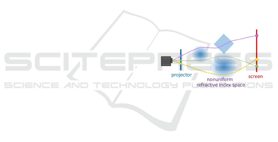
Figure 1: Recovery of 3D refractive index distribution of
nonuniform refractive index space.
2016). However, because of the complex nature of
refraction, these methods suffer from several strong
restrictions. Many of them are based on the assump-
tion that the light refracts only once or twice (Murase,
1990; Tian and Narasimhan, 2009; Xue et al., 2014;
Qian et al., 2016; Wetzstein et al., 2014), several are
based on the assumption that the refractive index of
the transparent object is known beforehand (Murase,
1990; Wetzstein et al., 2014), and almost all are based
on the assumption that there is a distinct boundary
for the refractive index, i.e. the object boundary, in
the 3D space (Murase, 1990; Morris, 2007; Tian and
Narasimhan, 2009; Wetzstein et al., 2014; Qian et al.,
2016; Wu. et al., 2018). Hence, these methods cannot
be used for recovering the 3D structure of a nonuni-
form refractive index distribution in 3D space.
On the other hand, in the field of fluid dynamics,
several methods have been developed for visualizing
and recovering the 3D distribution of the refractive
index in gas (Goldhahn and Seume, 2007; Atcheson
et al., 2008; Ramanah et al., 2007; Stryczniewicz,
654
Higuchi, T., Sakaue, F. and Sato, J.
Recovering 3D Structure of Nonuniform Refractive Space.
DOI: 10.5220/0008940106540663
In Proceedings of the 15th International Joint Conference on Computer Vision, Imaging and Computer Graphics Theor y and Applications (VISIGRAPP 2020) - Volume 4: VISAPP, pages
654-663
ISBN: 978-989-758-402-2; ISSN: 2184-4321
Copyright
c
 2022 by SCITEPRESS – Science and Technology Publications, Lda. All rights reserved

2018). However, these methods are specialized for
gas flows, for which the change in refractive index is
very small, and are based on the assumption that the
light ray path can be approximated by a straight line
in the refractive medium. Thus, if we consider the
reconstruction of a larger variation in the refractive
index in 3D space, such as the refractive index varia-
tion for solid and liquid objects, these methods are no
longer applicable.
Therefore, in this paper, we describe the challenge
of recovering an arbitrary refractive index distribution
in 3D space and propose a method for recovering a
fairly large variation in the refractive index distribu-
tion in a 3D space in which there are both gradual
and abrupt changes in the refractive indices. For this
objective, we project light rays from projectors and
observe the points of light on a screen by using cam-
eras, as shown in Fig. 1. The position of each point
on the screen depends on the refractive index of every
point on the corresponding light ray path. Hence, the
position of a point on the screen includes information
about the refractive index at all points along the path.
Thus, we project a large number of light rays from
a single or multiple projectors toward a nonuniform
refractive index space and reconstruct the 3D refrac-
tive index distribution of the space from their points
on the screen. However, if we have a large variation
in the distribution, the reconstruction is very difficult.
Thus, we propose an efficient two-step method that
combines a linear model and a non-linear model of
the light ray paths.
Since the boundary of the refractive index distri-
bution is considered to be the boundary of a transpar-
ent object, the recovery of the 3D refractive index dis-
tribution can be considered the reconstruction of the
whole 3D structure of a transparent scene.
2 RELATED WORK
Many methods have been reported for reconstructing
transparent objects. However, since the light transport
of typical transparent objects is very complicated, all
of the existing methods have limited applicability.
Murase (Murase, 1990) pioneered a method for
recovering the 3D shape of the surface of water in
a tank from the image distortion of the texture on
the bottom plane. Since then, the recovery of a wa-
ter surface has been studied extensively. Tian and
Narasimhan (Tian and Narasimhan, 2009) proposed
a method for recovering the shape of the water sur-
face and the texture of the bottom plane simultane-
ously. Morris and Kutulakos (Morris and Kutulakos,
2005) proposed a method for recovering an unknown
refractive index and the surface shape of water using
a known background pattern.
In the case of a water surface, the number of re-
fractions is limited to one. However, solid transparent
objects such as a glass accessory have more than one
refraction, so recovering their surface shape is more
difficult. Kutulakos and Steger (Kutulakos and Ste-
ger, 2005) investigated the feasibility of reconstruc-
tion under light ray refractions, and showed that three
views are enough for recovering the light paths for
up to two refractions. Qian et al. (Qian et al., 2016)
used constraints on position and normal orientation at
each surface point for recovering a 3D shape for up
to two refractions. Kim et al. (Kim et al., 2017) pro-
posed a method for recovering symmetric transparent
objects when there are more than two refractions. For
recovering nonsymmetric objects with more than two
refractions, Wu et al. (Wu. et al., 2018) proposed a
shape-recovery method based on both ray constraints
and silhouette information. Using both space curving
and ray tracing, their method can reconstruct complex
nonsymmetric transparent objects from images.
Although these methods improve the shape recov-
ery of solid transparent objects drastically, they are all
based on the assumption that the light rays are piece-
wise linear and that they refract only at the surface of
objects, more precisely at the boundary between me-
dia. The media type is unlimited, but each medium
must be homogeneous and have a constant refractive
index. This assumption is valid for most solid objects.
However, if we consider more complex objects, such
as heated air or a liquid mixture, these methods are
no longer applicable. Xue et al. (Xue et al., 2014)
proposed a method for recovering the nonuniform re-
fractive index in gas. However, the gas is assumed to
be a thin film, so the incoming light refracts only once
in the gas.
For visualizing and recovering nonuniform refrac-
tive index distributions, such as that in a gas flow,
the background oriented schlieren (BOS) method has
been proposed in the field of fluid dynamics (Dalziel
et al., 2000; Raffel et al., 2000). The BOS method
first obtains the displacement vectors of a random dot
pattern behind nonuniform refractive media and then
uses these vectors as the integrals of refraction in the
viewing direction for tomographic reconstruction of
the refractive index distribution (Goldhahn and Se-
ume, 2007; Raffel, 2015). Several variants of the
BOS method have been proposed that improvethe ac-
curacy of gas flow estimation. Venkatakrishnan and
Meier (Venkatakrishnan and Meier, 2004) improved
the stability of the BOS method by assuming that
the objective gas flow is axisymmetric. Atcheson et
al. (Atcheson et al., 2008) proposed a linear method
Recovering 3D Structure of Nonuniform Refractive Space
655

for estimating the gradient field of the refractive index
distribution. However, their method requires a com-
plex post integration to recover the refractive index
distribution from its gradient field, and this post in-
tegration is based on the assumption that the bound-
ary of the objective gas flow is available. Although
these assumptions may be valid in the field of gas flow
estimation, they are obviously not valid for cases in
which the refractive index distribution is not symmet-
ric and does not have a distinct distribution boundary,
such as heat haze on a road. Moreover, since these
methods use tomographic reconstruction, light ray re-
fraction is assumed to be very small, so the light path
can be approximated by a straight line. This approx-
imation is valid if the refractive media is gas, as is
assumed in these methods. However, if we want to
reconstruct refractive indices with larger variations,
such as for nonuniform solid or liquid objects, straight
ray approximation is no longer valid, and the BOS
methods suffer from large errors in 3D reconstruction.
Therefore, we present in this paper a novelmethod
for recovering nonuniform refractive index distri-
butions that may include both gradual and abrupt
changes in the refractive index. Unlike the existing
methods in computer vision, our method does not
need to limit the number of refractions, its applica-
tion is not limited to uniform objects, and there is no
need to know the refractive index of the media before-
hand. Thus, it can be applied to the 3D reconstruction
of non-uniform refractive media, such as heat haze.
Also, our method does not depend on the assumption
of symmetry in the refractive index distribution or the
existence of a distribution boundary, unlike the BOS
methods in the field of gas flow estimation.
3 PARAMETRIC
REPRESENTATION OF
NONUNIFORM REFRACTIVE
MEDIA
For reconstructing the refractive indices of the whole
3D space efficiently, here we represent the refractive
index distribution parametrically by using a Fourier
series representation, i.e., Fourier basis functions and
their coefficients. Use of Fourier basis functions and
their coefficients enables the refractive index distribu-
tion to be represented sparsely by using a small num-
ber of non-zero parameters.
Suppose we have a 1D continuous signal n(x) that
spans from x = 0 to x = X. By considering it as a
repetitive signal with a period of [0, X], we can repre-
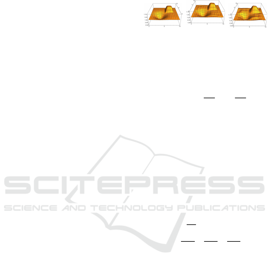
(a) original
(b) 101
coefficients
(c) 40 coefficients
Figure 2: Sparse Fourier series representation of refractive
index distribution. Vertical axis shows refractive index at
each point in 2D space. Both gradual and abrupt changes in
refractive index distribution can be represented by using a
small number of coefficients, as shown in (b) and (c).
sent it by using a Fourier series up to the Nth order:
n(x) = a
0
+
N
∑
i=1
a
i
cos
2iπx
X
+ b
i
sin
2iπx
X
(1)
where a
0
and a
i
, b
i
(i = 1, · ·· , N) are the Fourier co-
efficients, and these 2N + 1 coefficients represent the
shape of the signal. In general, many coefficients in a
i
and b
i
are close to 0, so the signals can be represented
by using a small number of coefficients.
By extending the 1D Fourier series representa-
tion, we can describe the refractive index distribution
n(x, y, z) in 3D space as
n(x, y, z) = Ba (2)
where a = [a
000
, · ·· , a
2N,2N,2N
]
⊤
represents a (2N +
1)
3
vector consisting of the Nth order Fourier coef-
ficients on the x, y, and z axes, and B represents a
(2N + 1)
3
vector consisting of 3D Fourier basis func-
tions on the x, y, and z axes:
B =

1, cos
2πx
X
, · ·· ,
sin
2Nπx
X
sin
2Nπy
Y
sin
2Nπz
Z

(3)
where X, Y, and Z denote the size of the refractive
index space along the x, y, and z axes, respectively.
The reconstruction of the 3D refractive index distri-
bution can then be considered as the estimation of the
(2N + 1)
3
Fourier coefficients, a
ijk
, in a.
For representing the abrupt changes in the refrac-
tive index distribution, we need high order terms in
the Fourier coefficients vector a, and hence we need
to choose a large number as N. However, even in such
cases, many coefficients in a are close to zero, so vec-
tor a is sparse. Thus, we estimate vector a by using a
sparse estimation method in a later section.
Fig. 2 shows an example of a 2D refractive in-
dex distribution represented by Fourier coefficients in
which both gradual and abrupt changes in the refrac-
tive index exist in the space. As shown in this figure,
a small number of Fourier coefficients is enough for
representing complex distributions.
VISAPP 2020 - 15th International Conference on Computer Vision Theory and Applications
656

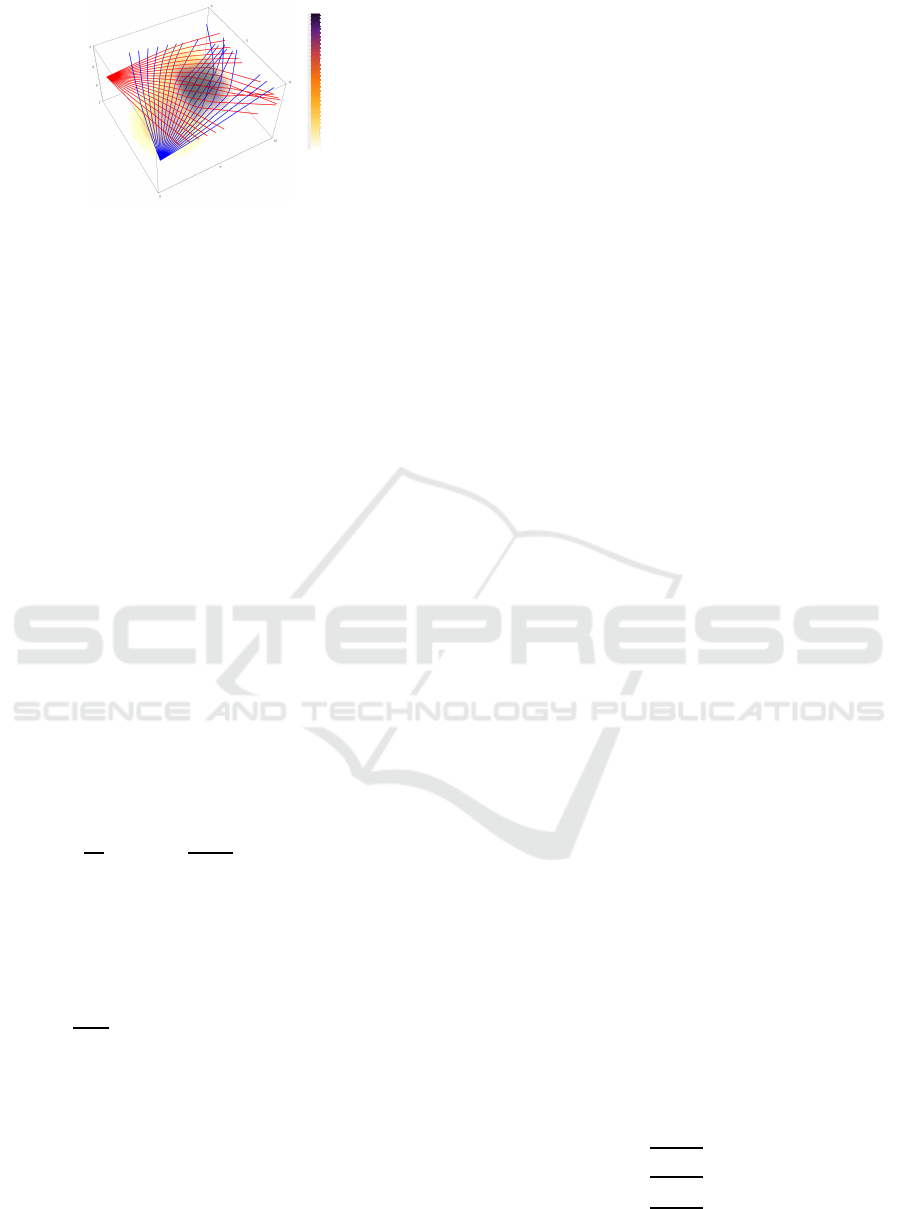
1.025
1.050
1.075
1.100
1.125
1.150
1.175
Figure 3: Ray tracing based on ray equation, Eq. (4). Light
rays bend gradually or abruptly in accordance with gradient
of refractive index field. Straight ray assumption used in
BOS method is not valid under such strong refraction.
4 MODELING RAY REFRACTION
We next consider light ray refraction in nonuniform
refractive index media.
If we have a glass object in air, there is a dis-
tinct boundary surface for the refractive index. In this
case, the refraction of a light ray at the boundary sur-
face can be described by Snell’s law (Born and Wolf,
1980). However, if the refractive index changes con-
tinuously, such as for air with a nonuniform tempera-
ture, Snell’s law is no longer applicable. In this case,
the orientation of each light ray changes continuously
in accordance with the refractive index distribution,
so the change in orientation can be described by us-
ing the ray equation.
Suppose we have a nonuniform refractive index
space. Let n(x) be its refractive index at point x =
[x, y, z]
⊤
. Then, a light ray passing through x can be
described by the following ray equation (Born and
Wolf, 1980):
d
ds

n(x(s))
dx(s)
ds

= ∇n(x(s)) (4)
where s represents the position on the light ray, and
∇n(x) denotes the gradient of n at point x.
Since Eq. (4) is a 2nd order differential equation,
a light ray path can be obtained by solving the differ-
ential equation using incident position x(0) and ori-
entation
dx(0)
dt
of the light ray at s = 0. The solution of
the differential equation can be obtained by using the
Runge-Kutta method. Then, the position of the light
ray at the screen can be derived by ray tracing using
Eq. (4).
Fig. 3 shows an example of light rays in a nonuni-
form refractive index space that were derived from
Eq. (4). The orientation of each light ray changes
gradually or abruptly in accordance with the changes
in the refractive index, so the straight ray assumption
used in the BOS methods is not valid in this case.
5 RECONSTRUCTION OF
REFRACTIVE INDEX
DISTRIBUTION
We next describe our method for reconstructing 3D
refractive index distributions from light ray positions
on a screen. We calibrate the projectors, cameras, and
the screen geometrically beforehand, so the light rays
projected from the projectors and the screen points
observed by the cameras are described in a single con-
sistent set of 3D coordinates.
The fundamental strategy of our method is to find
the coefficient vector a of the refractive index distri-
bution that minimizes the error between light rays ob-
served by the cameras and light rays synthesized from
vector a by using the ray equation, Eq. (4). However,
this minimization problem is easily trapped by local
minima in general. Therefore, we propose an efficient
two-step method for estimating coefficient vector a.
We describe each step below.
5.1 Linear Estimation of Initial Value
We first estimate Fourier coefficient vector a by us-
ing a linear approximation of the light ray model.
This is similar to the method proposed by Atcheson
et al. (Atcheson et al., 2008) but is different in a very
important way. Atcheson et al. used a linear basis
model to represent the gradient field, ∇n(x, y, z), of
the refractive index, n(x, y, z), and estimated the co-
efficients of the model. After estimating the gradi-
ent field, they integrated the gradient field to estimate
the refractive index distribution. However, this inte-
gration is noise sensitive, so it is not easy to obtain
good results (Atcheson et al., 2008). Furthermore,
it requires a distinct boundary for the gradient field,
which is not always present in general cases. Thus,
here we derive a method for estimating the refractive
index distribution directly by using linear estimation.
Since this approach does not require integration of the
gradient field afterwards, computation is very stable
and boundary information is not required.
Unlike Atcheson et al. (Atcheson et al., 2008),
we use a linear basis model to represent the refrac-
tive index distribution directly, as shown in Eq. (2).
Then, by taking its derivative, we can obtain the gra-
dient field ∇n(x, y, z) of the refractive index distribu-
tion n(x, y, z):
∇n(x, y, z) =



∂n(x,y,z)
∂x
∂n(x,y,z)
∂y
∂n(x,y,z)
∂z



=


B
x
B
y
B
z


a (5)
where B
x
, B
y
, and B
z
denote the derivative of B with
respect to x, y, and z, respectively.
Recovering 3D Structure of Nonuniform Refractive Space
657

Now, since the first term of B is equal to 1, the first
terms of B
x
, B
y
, and B
z
are equal to 0. Thus, Eq. (5)
can be rewritten as:
∇n(x, y, z) =


B
′
x
B
′
y
B
′
z


a
′
(6)
where a
′
, B
′
x
, B
′
y
, and B
′
z
are vectors made by dropping
the first term in a, B
x
, B
y
, and B
z
, respectively.
The important point here is that coefficients a in
Eq. (2) are identical with coefficients a in Eq. (5), so
they are identical with a
′
in Eq. (6) except the first
term in vector a. On the basis of this observation,
we next propose a linear method for estimating coef-
ficients a of refractive index distribution n(x, y, z) di-
rectly by using its gradient field, ∇n(x, y, z).
By taking the line integral of Eq. (4) along light
ray path C in the nonuniform refractive index space,
we have the relationship:
n(x)
dx
ds
=
Z
C
∇n(x)ds+ d
0
(7)
where d
0
is the input orientation of the light ray.
dx
ds
in Eq.(7) represents the orientation of light ray
d
1
at the end of integral curve C, so it corresponds to
the output orientation of the light ray. Assuming that
the refractive index at the boundary of the observation
area is 1.0 and substituting Eq. (6) into Eq. (7), we
have the relationship:
d
1
− d
0
=
Z
C


B
′
x
B
′
y
B
′
z


a
′
ds (8)
Although the refractive index distribution is not
uniform in the observation area, its coefficients a do
not change in this area. Thus, Eq. (8) can be rewritten
as:
∆d = Ma
′
(9)
where ∆d = d
1
− d
0
, and M is a 3 × ((2N + 1)
3
−
1) matrix derived by integrating the derivative of the
basis functions:
M =
Z
C


B
′
x
B
′
y
B
′
z


ds (10)
Suppose we project L light rays from a single or
multiple projectors. We then have:



∆d
1
.
.
.
∆d
L



=



M
1
.
.
.
M
L



a
′
(11)
where ∆d
i
denotes ∆d of the ith light ray, and M
i
de-
notes matrix M computed from the ith light ray path
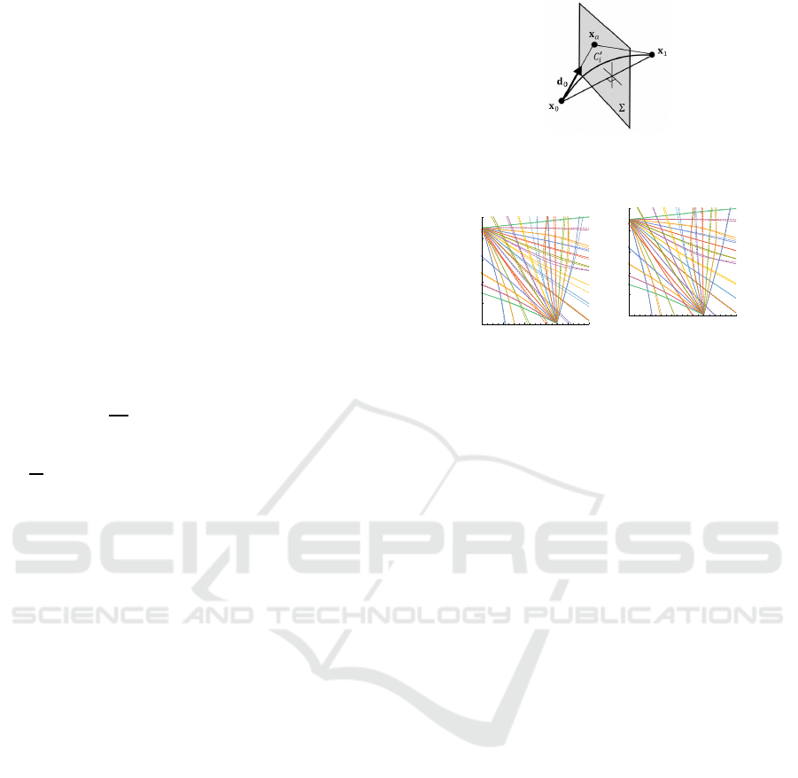
Figure 4: Integral curve C
′
i
defined by quadratic Bezier
curve generated by three basis points, x
0
, x
1
, and x
a
which
is on symmetric plane Σ and in direction d
0
.
0 2 4 6 8 10
0
2
4
6
8
10
(a) sparse linear
0 2 4 6 8 10
0
2
4
6
8
10
(b) fine
estimation
Figure 5: Light rays obtained using sparse linear estimation
and fine estimation. Solid lines and dashed lines show es-
timated rays and ground truth rays, respectively. Obtained
rays converge to ground truth rays after fine estimation.
C
i
. Thus, if we know light ray path C
i
(i = 1, ··· , L),
matrix M
i
(i = 1, ·· · , L) can be computed, and coeffi-
cient vector a
′
can be estimated linearly from Eq. (11).
However, light ray path C
i
in a nonuniform re-
fractive index space is not known beforehand. There-
fore, we approximateit by using a quadraticcurvethat
passes through input point x
0
and output point x
1
in
the observation area and has orientation d
0
at the input
point. Since there exists an infinite number of such
quadratic curves, we choose a symmetric one with re-
spect to the input and output points. Such a quadratic
curve, C
′
i
, can be obtained as a quadratic Bezier curve
whose three basis points are input point x
0
, output
point x
1
, and intersection point x
a
between an input
light ray line and a symmetric plane perpendicularto a
line segment x
0
x
1
, as shown in Fig. 4. Once quadratic
curve C
′
i
is computed, matrix M
i
(i = 1, ·· · , L) can
be obtained from Eq. (10). We can also compute out-
put orientation d
1
by taking the derivative of C
′
with
respect to s. Then, Fourier coefficient a
′
of the refrac-
tive index distribution can be estimated linearly from
Eq. (11).
However, this linear method does not work well
since Fourier coefficient vector a
′
of a refractive in-
dex distribution is sparse in general, and the coeffi-
cients estimated from Eq. (11) fit not only the objec-
tive distribution but also image noises. If we estimate
only low order terms of a
′
, we can avoid this prob-
lem, but the abrupt changes in the distribution can-
not be recovered. Therefore, we estimate coefficient
vector a
′
by using a sparse estimation method under
linear constraints without reducing the order of the
VISAPP 2020 - 15th International Conference on Computer Vision Theory and Applications
658

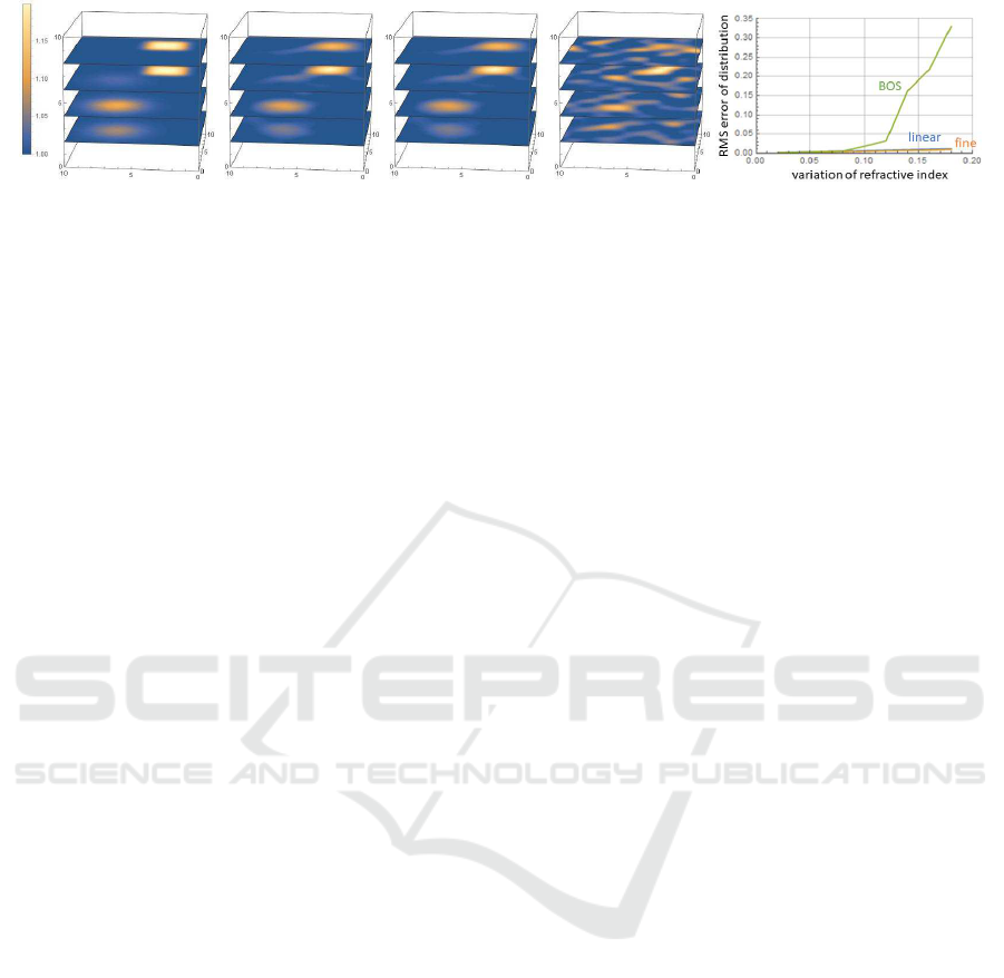
(a) ground truth
(b) linear est. (c) fine est. (d) BOS method
(e) RMSE
Figure 6: Cross-sectional views of refractive index distributions obtained using proposed method and existing BOS method
in synthetic image experiments: (b) and (c) show distributions obtained using our sparse linear estimation and fine estimation,
respectively. For comparison, (d) shows result using BOS method (Goldhahn and Seume, 2007). (e) shows relationship
between magnitude of variation of refractive index distribution and RMS error of reconstructed distribution.
Fourier coefficients. We use Lasso (Tibshirani, 1996)
and estimate sparse vector a
′
by solving the following
minimization problem:
ˆ
a
′
= argmin
a
′
L
∑
i=1
k∆d
i
− M
i
a
′
k
2
+ λka
′
k
1
(12)
where k · k
1
denotes an L
1
norm, and λ denotes its
weight. Once sparse Fourier coefficients a
′
are esti-
mated, the refractive index distribution n(x, y, z) can
be obtained from Eq. (2). Since the first term a
000
of
the Fourier coefficients is indeterminate in this stage,
we set a
000
= 1 temporarily, and it is estimated in the
following fine estimation stage.
The sparse linear method described in this sec-
tion can estimate the refractive index distribution di-
rectly from the observed screen points, and it does
not require post integration of the gradient field of
the refractive index, unlike the method of Atcheson
et al. (Atcheson et al., 2008). Thus, it is efficient and
computationally stable.
5.2 Fine Estimation of Distribution
By using the sparse linear method described in sec-
tion 5.1, we can roughly estimate refractive index dis-
tributions. However, the estimated distributions may
have errors since the integral curve C
′
used in the lin-
ear model may deviate somewhat from the true light
ray path. Thus, we next estimate the light ray path and
the refractive index distribution simultaneously min-
imizing the observation error. The refractive index
distribution estimated from the linear model is used
as the initial value of this minimization.
Suppose we project L light rays from a single or
multiple projectors toward a nonuniformrefractive in-
dex space. Let x
i
be the observed position of the ith
light ray on the screen. We compute the light ray posi-
tion,
ˆ
x
i
(a), on the screen by using ray tracing based on
Eq. (4) in a refractive index distribution represented
by Eq. (2). Then, we find the Fourier coefficients a
that minimize
∑
L
i=1
kx
i
−
ˆ
x
i
(a)k
2
.
In this estimation, we also want to fix the refrac-
tive index to 1.0 at the boundary of the observation
area. This is achieved by minimizing cost function:
b(a) =
Z
B
k1− n(a)k
2
ds (13)
where B denotes the boundary line of the observation
area.
For estimating the sparse coefficients, we add the
L
1
norm of vector a to the cost function. Thus, we
estimate coefficients a of the refractive index distribu-
tion by solving the following minimization problem:
ˆ
a = argmin
a
L
∑
i=1
kx
i
−
ˆ
x
i
(a)k
2
+ µb(a) + λkak
1
(14)
where µ denotes the weight of the boundary error.
We used the steepest descent method to minimize
the cost function and used coefficient vector a esti-
mated using the method in section 5.1 as the initial
value of this minimization problem. Once coefficients
a are estimated from Eq. (14), the refractive index dis-
tribution n(x, y, z) can be obtained from Eq. (2).
Fig. 5 shows the rays estimated using the sparse
linear method described in section 5.1 and the fine es-
timation method described in section 5.2. The rays af-
ter fine estimation are almost identical to the ground
truth rays, whereas those from sparse linear estima-
tion deviate somewhat from the ground truth rays.
5.3 Recovery of Time Varying
Distribution
We next extend our method for estimating time vary-
ing distributions. In most cases, the change in the dis-
tribution is continuous. Thus, we enhance the stabil-
ity of the recovery by adding smoothness constraints
in the time domain. Suppose we have a time series
of observations, x
ij
( j = 1, ··· , T). We estimate the
Recovering 3D Structure of Nonuniform Refractive Space
659

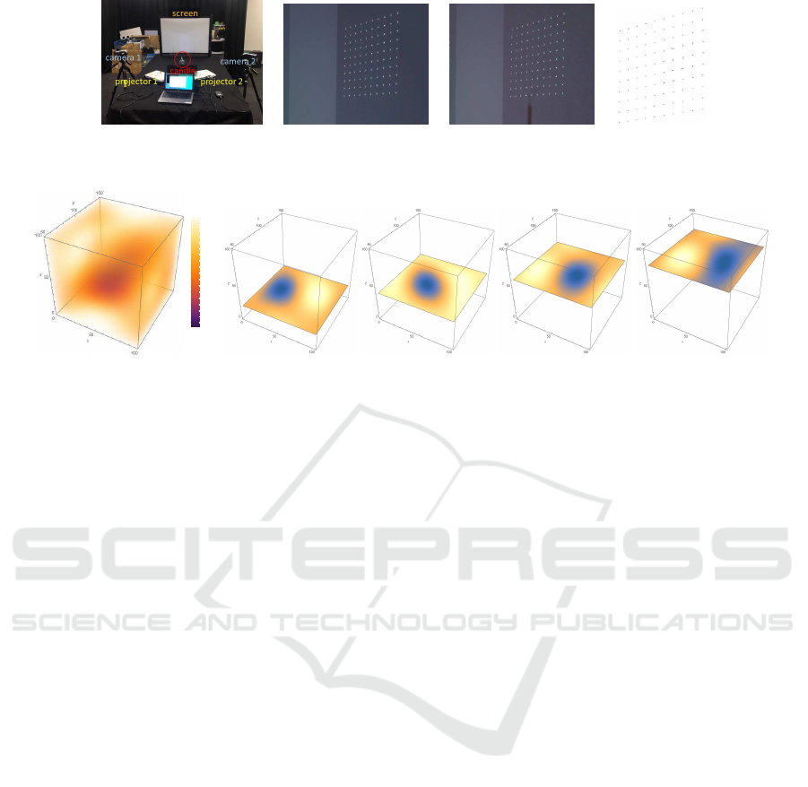
(a) experimental setup (b) without candle (c) with candle (d) deviation
Figure 7: Experimental setup and light rays projected on screen. (d) shows deviation in light rays caused by heated air.
(a) refractive index
distribution
0.99980
0.99990
1.00000
1.00010
(b) z = 20 (c) z = 40 (d) z = 60 (e) z = 80
Figure 8: Refractive index distribution reconstructed with proposed method and cross-sectional views on four horizontal
planes.
time series of coefficient vectors a
j
( j = 1, · ·· , T) as
follows:
{
ˆ
a
1
, · ·· ,
ˆ
a
T
} = argmin
{a
1
,···,a
T
}
T
∑
j=1
L
∑
i=1
kx
ij
−
ˆ
x
i
(a
j
)k
2
+µb(a
j
) + λka
j
k
1
+ κL (a
j
)(15)
where T denotes the number of time instants in the
sequential observations, and L (a
j
) denotes a discrete
Laplacian of a
j
along the time axis. The smoothness
is controlled by adjusting weight κ.
Once the time series of coefficients is obtained,
the change in the refractive index distribution n
j
can
be recovered as follows:
n
j
(x, y, z) = Ba
j
( j = 1, ·· · , T) (16)
In this way, we can recover a dynamic 3D refractive
index space, such as heated air or mixture of different
types of liquid.
6 EXPERIMENTS
6.1 Synthetic Image Experiment
To evaluate the performance of our proposed method,
we first tested it by using synthetic images generated
by projecting light rays into a synthetic nonuniform
refractive index space. In this experiment, we used
a nonuniform distribution that included both gradual
and abrupt changes in the refractive index, as shown
in Fig. 6 (a). The refractive index varied from 1.0 to
1.16. Since the variation of the refractive index of
gas is 1.0 − 1.0005, the variation in Fig. 6 (a) is quite
large.
In our estimation, the refractive index distribution
was modeled by a 6th order Fourier series, resulting
in 13
3
= 2197 parameters for coefficient vector a. Us-
ing three projectors, we projected 108 rays of light in
total. Then, 108 projected points on the screen were
used for estimation.
Since each point on the screen provides three con-
straints on the distribution, we had 108×3= 324 con-
straints in total. Although the number of parameters
to be estimated exceeds the number of constraints ob-
tained from the observation, our method can still re-
cover the distribution since the coefficients are sparse
and our method uses sparse estimation.
Fig. 6 (b) and (c) show the refractive index distri-
butions estimated using our sparse linear estimation
and fine estimation, respectively. The linear estima-
tion deriveda rough estimation of the distribution, and
the fine estimation improved its accuracy. For com-
parison, the distribution obtained using the existing
BOS method (Goldhahn and Seume, 2007) is shown
in Fig. 6 (d). The BOS method could not recover the
original distribution accurately, and there were many
artifacts in the distribution. This is because the change
in the refractive index was fairly large (1.0− 1.16), so
the straight line assumption used in the BOS method
was invalid.
Fig. 6 (e) shows the relationship between the mag-
VISAPP 2020 - 15th International Conference on Computer Vision Theory and Applications
660

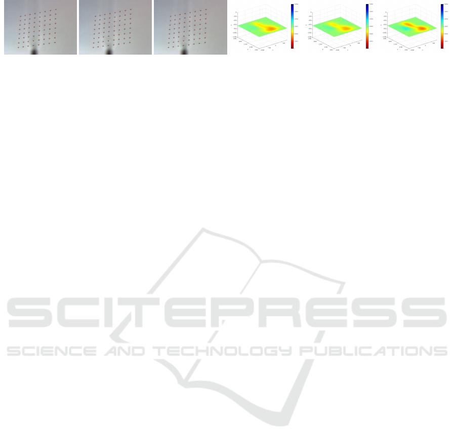
(a) time 1 (b) time 2 (c) time 3 (d) time 1 (e) time 2 (f) time 3
Figure 9: Three sequential images of rays on screen taken with camera at 30 fps, and cross-sectional view of reconstructed
refractive index distribution at each time instant.
nitude of the variation of refractive index distribution
and the RMS error of the reconstructed distribution.
As we can see in this graph, the accuracy of the BOS
method degrades rapidly under large variations of the
refractive index while the proposed method is accu-
rate even under large variations.
6.2 Real Image Experiment
We next evaluated the performance of our proposed
method by using real images obtained from nonuni-
form refractive media. We positioned two projec-
tors, two cameras, and a screen as shown in Fig. 7
(a) and reconstructed the nonuniform refractive me-
dia between the projectors and screen.
The thermal space around a candle flame was used
as the nonuniform refractive index space. As men-
tioned above, the refractive index of air varies with
the temperature. Thus, the 3D refractive index dis-
tribution of air heated by a candle flame is nonuni-
form. Moreover, since the temperature changes over
time, the refractive index distribution of heated air
also changes over time. We thus reconstructed the
refractive index distribution at each time instant and
recovered the dynamic change in the refractive index
distribution.
We projected 64 rays from each projector toward
the heated air and observed the resulting 128 points on
the screen by capturing camera images at each time
instant. Fig. 7 (b) and (c) show examples of points
observed with and without the candle flame. The de-
viations in the light rays caused by the heated air are
shown in Fig. 7 (d).
Again, since each point on the screen provides
three constraints on the distribution, we had 384 con-
straints in total. We used 4th order Fourier coeffi-
cients to represent the distribution, so there was a total
of 729 parameters for coefficient vector a. Again, the
number of parameters exceeded the number of con-
straints obtained from the observation, but our method
still recovered the distribution because of the sparse
estimation.
Fig. 8 (a) shows the 3D refractive index distribu-
tion of heated air reconstructed using the proposed
method from the images in Fig. 7. Fig. 8 (b) through
(e) show cross-sectional views of the distribution for
four horizontal planes. These results show that the
nonuniform refractive index distribution of heated air
can be recovered by using the proposed method.
We next recoveredthe refractiveindex distribution
of a dynamically changing thermal space. Since the
proposed method can recover the refractive index dis-
tribution from a single time image, it is possible to
recover the temporal change in the refractive index,
as described in section 5.3.
Fig. 9 shows three sequential images of rays on
the screen captured with a camera at 30 fps and cross-
sectional views of estimated changes in the refractive
index distribution at three time instants. It shows that
the refractive index distribution in a thermal space
changes over time and that our method can recover
these dynamic changes. These results demonstrate
that, by using the proposed method, we can recon-
struct the 3D structure of a dynamically changing
transparent space.
6.3 Various Nonuniform Distributions
We next evaluated the performance of our method for
various nonuniform refractive index distributions by
using synthetic images. As shown in the first row
of Fig. 10, we tested not only gradual changes in
the refractive index but also abrupt changes, holes,
and nested distributions. The second row in Fig. 10
shows the distributions estimated using our method,
and the third row shows the results for the BOS
method (Goldhahn and Seume, 2007). The table com-
pares the accuracy of these two methods numerically.
These results demonstrate that the proposed method
outperforms the BOS method. In particular, the BOS
method completely fails when the variation of distri-
bution is large or abrupt, while the proposed method
provides us good results even in such cases.
7 CONCLUSION
We have developeda method for recovering the whole
refractive index distribution in a 3D space. The re-
fractive index distribution is represented parametri-
Recovering 3D Structure of Nonuniform Refractive Space
661

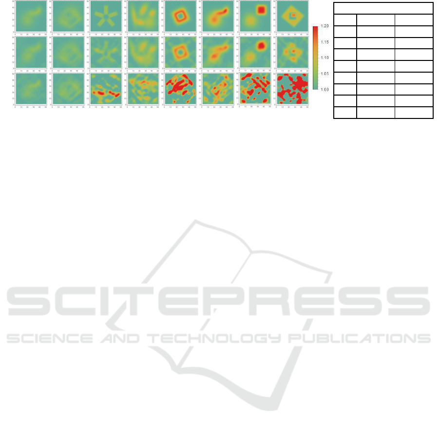
BOS proposed
(a) (b) (c) (d) (e) (f)
(g)
(h)
RMS Error
ours BOS
(a) 0.0028 0.0038
(b) 0.0037 0.0051
(c) 0.0133 0.0730
(d) 0.0107 0.0426
(e) 0.0144 0.1516
(f) 0.0130 0.0546
(g) 0.0124 0.1677
(h) 0.0175 0.6445
Figure 10: Performance of proposed method for various nonuniform refractive index distributions. First row shows ground
truth distributions, and second and third rows show distributions estimated using proposed method and BOS method (Gold-
hahn and Seume, 2007), respectively. Table shows corresponding RMS errors in recovered distributions. If variation of
distribution is small, both methods provide us good results. However, if variation of distribution is large or abrupt, BOS
method fails whereas our proposed method provides us good results.
cally and sparsely by using Fourier series represen-
tation. The complex refractive index distribution is
reconstructed by combining a linear model and a non-
linear model of the light ray paths. The linear model
is used to directly estimate the refractive index distri-
bution simply by solving linear equations with sparse-
ness constraints. The non-linear model is used to im-
prove the accuracy of the distribution. Unlike exist-
ing methods, our method can recover the refractive
index distribution of the whole 3D space, even if the
space includes both gradual and abrupt changes in the
refractive index. It can thus be used to recover the
3D structure of complex transparent scenes, such as
heated air.
Evaluation of the proposed method using both
synthetic and real images demonstrated its ability to
reconstruct the refractive index distribution of a dy-
namically changing nonuniform refractive space.
Recovering the whole 3D structure of a transpar-
ent space is a very tough problem, and we have pre-
sented a method for efficiently solving this problem.
REFERENCES
Agarwal, S., Snavely, N., Simon, I., Sietz, S., and Szeliski,
R. (2009). Building Rome in a day. In Proc. IEEE
International Conference on Computer Vision.
Atcheson, B., Ihrke, I., Heidrich, W., Tevs, A., Bradley, D.,
Magnor, M., and Seidel, H.-P. (2008). Time-resolved
3D capture of non-stationary gas flows. ACM Trans-
actions on Graphics, 27(5).
Barron, J. and Malik, J. (2015). Shape, illumination, and re-
flectance from shading. IEEE Transaction on Pattern
Analysis and Machine Intelligence, 37(8):1670–1687.
Born, M. and Wolf, E. (1980). Principles of optics: elec-
tromagnetic theory of propagation, interference and
diffraction of light. Elsevier.
Dalziel, S., Hughes, G., and Sutherland, B. (2000). Whole-
field density measurements by ’synthetic schlieren’.
Experiments in Fluids, 28(4):322–335.
Faugeras, O. and Luong, Q.-T. (2004). The Geometry of
Multiple Images. MIT Press.
Goldhahn, E. and Seume, J. (2007). The background ori-
ented schlieren technique: sensitivity, accuracy, reso-
lution and application to a three-dimensional density
field. Experiments in Fluids, 43(2–3):241–249.
Hartley, R. and Zisserman, A. (2000). Multiple View Geom-
etry in Computer Vision. Cambridge University Press.
Horn, B. and Brooks, M. (1989). Shape from Shading. MIT
Press.
Ikeuchi, K. (1981). Determining surface orientations of
specular surfaces by using the photometric stereo
method. IEEE Transactions on Pattern Analysis and
Machine Intelligence, 3(6):661–669.
Inoshita, C., Mukaigawa, Y., Matsushita, Y., and Yagi, Y.
(2012). Shape from single scattering for translucent
objects. In Proc. European Conference on Computer
Vision, pages 371–384.
Kim, J., Reshetouski, I., and Ghosh, A. (2017). Acquiring
axially-symmetric transparent objects using single-
view transmission imaging. In Proc. IEEE Conference
on Computer Vision and Pattern Recognition, pages
1484–1492.
Kutulakos, K. and Steger, E. (2005). A theory of refractive
and specular 3d shape by light-path triangulation. In
IEEE International Conference on Computer Vision,
volume 2, pages 1448–1455.
Morris, N. (2007). Reconstructing the surface of inhomo-
geneous transparent scenes by scatter-trace photogra-
phy. In IEEE International Conference on Computer
Vision.
Morris, N. and Kutulakos, K. (2005). Dynamic refraction
stereo. In IEEE International Conference on Com-
puter Vision, volume 2, pages 1573–1580.
Murase, H. (1990). Surface shape reconstruction of an un-
dulating transparent object. In Proc. IEEE Interna-
tional Conference on Computer Vision, pages 313–
317.
VISAPP 2020 - 15th International Conference on Computer Vision Theory and Applications
662

Nishino, K., Subpa-asa, A., Asano, Y., Shimano, M., and
Sato, I. (2018). Variable ring light imaging: Capturing
transient subsurface scattering with an ordinary cam-
era. In Proc. European Conference on Computer Vi-
sion, pages 598–613.
Owens, J. (1967). Optical refractive index of air: depen-
dence on pressure, temperature and composition. Ap-
plied Optics, 6(1).
Qian, Y., Gong, M., and Yang, Y. (2016). 3D reconstruc-
tion of transparent objects with position-normal con-
sistency. In Proc. IEEE Conference on Computer Vi-
sion and Pattern Recognition, pages 4369–4377.
Raffel, M. (2015). Background-oriented schlieren (BOS)
techniques. Experiments in Fluids, 56(3).
Raffel, M., Richard, H., and Meier, G. (2000). On the ap-
plicability of background oriented optical tomography
for large scale aerodynamic investigations. Experi-
ments in Fluids, 28(5):477–481.
Ramanah, D., Raghunath, S., Mee, D., Rosgen, T., and
Jacobs, P. (2007). Background oriented schlieren
for flow visualisation in hypersonic impulse facilities.
Shock Waves, 17(1–2):65–70.
Stryczniewicz, W. (2018). Quantitative visualisation of
compressible flows. Transactions of the Institute of
Aviation, pages 132–141.
Tian, Y. and Narasimhan, S. (2009). Seeing through wa-
ter: Image restoration using model-based tracking. In
Proc. IEEE International Conference on Computer Vi-
sion, pages 2303–2310.
Tibshirani, R. (1996). Regression shrinkage and selection
via the lasso. Journal of the Royal Statistical Society.
Series B, 58(1):267–288.
Venkatakrishnan, L. and Meier, G. (2004). Density mea-
surements using the background oriented schlieren
technique. Experiments in Fluids, 37(2):237?–247.
Wetzstein, G., Heidrich, W., and Raskar, R. (2014).
Computational schlieren photography with light field
probes. International Journal of Computer Vision,
110(2):113–127.
Woodham, R. (1980). Photometric method for determin-
ing surface orientation from multiple images. Optical
Engineering, 19(I):139–144.
Wu., B., Zhou, Y., Qian, Y., Cong, M., and Huang, H.
(2018). Full 3d reconstruction of transparent objects.
ACM Transactions on Graphics, 37(4).
Xue, T., Rubinstein, M., Wadhwa, N., Levin, A., Durand, F.,
and Freeman, W. (2014). Refraction wiggles for mea-
suring fluid depth and velocity from video. In Proc.
European Conference on Computer Vision.
Recovering 3D Structure of Nonuniform Refractive Space
663