Deep Learning for Astronomical Object Classiﬁcation: A Case Study

Ana Martinazzo, Mateus Espadoto

and Nina S. T. Hirata

Institute of Mathematics and Statistics, University of S

ao Paulo, S

ao Paulo, Brazil

Keywords:

Deep Learning, Astronomy, Galaxy Morphology, Merging Galaxies, Transfer Learning, Neural Networks,

ImageNet.

Abstract:

With the emergence of photometric surveys in astronomy, came the challenge of processing and understanding

an enormous amount of image data. In this paper, we systematically compare the performance of ﬁve popular

ConvNet architectures when applied to three different image classiﬁcation problems in astronomy to deter-

mine which architecture works best for each problem. We show that a VGG-style architecture pre-trained on

ImageNet yields the best results on all studied problems, even when compared to architectures which perform

much better on the ImageNet competition.

1 INTRODUCTION

Traditionally, astronomers relied on spectroscopy to

gather data from objects in the sky, which is very

accurate, since it can collect data from thousands of

frequency bands in the electromagnetic spectrum, but

very time-consuming, since it usually works for a

single object at a time and requires longer exposure

times. In recent years, with advances in telescope

and sensor technology, there was a shift towards pho-

tometric surveys, where a trade-off was made: data

from only a few frequency bands are collected, typi-

cally less than a dozen, but for many objects at a time.

With this huge amount of data available, came the

problem of making sense of all of it, and this is where

machine learning (ML) comes into play. There are

many works on how to use ML in astronomy, like

(Ball and Brunner, 2010; Ivezi

c et al., 2014), but

many of them focus on processing astronomical cata-

log data, which is pre-processed data in table format

based on features extracted from photometric data. In

particular, there are quite a few works that address the

problem of object classiﬁcation, which can be of dif-

ferent types, such as star/galaxy classiﬁcation (Moore

et al., 2006) or galaxy morphology (Gauci et al.,

2010).

More recently, with the growing popularity of

Deep Learning techniques applied to images, fu-

eled by the development of the AlexNet architec-

ture (Krizhevsky et al., 2012), some works based on

https://orcid.org/0000-0002-1922-4309

https://orcid.org/0000-0001-9722-5764

Deep Learning for astronomy started to appear. Ex-

amples include star/galaxy classiﬁcation (Kim and

Brunner, 2016), galaxy morphology (Dieleman et al.,

2015) and merging galaxies detection (Ackermann

et al., 2018), all based on images, and galaxy classiﬁ-

cation based on data from radio telescopes (Aniyan

and Thorat, 2017). However, as we understand it,

Deep Learning techniques have not yet been system-

atically explored in astronomy. This might have to do

with the fact that typically a large amount of labeled

data is required to train deep neural networks. Label-

ing astronomical data is costly, as it requires expert

knowledge or crowdsourcing efforts, such as Galaxy

Zoo (Lintott et al., 2008).

To help alleviate the lack of labeled data inher-

ent to many ﬁelds, the idea of Transfer Learning (Pan

and Yang, 2009) was applied to Deep Learning (Ben-

gio, 2012). Deep neural networks trained with huge

datasets such as ImageNet (Deng et al., 2009), which

contains millions of images, can be used as generic

image feature extractors, or be ﬁne-tuned for particu-

lar, much smaller datasets.

In this paper, we present a systematic study of

Deep Learning models applied to different image

classiﬁcation problems in astronomy. We compare

the accuracy obtained by ﬁve popular models in the

literature, when trained from scratch or pre-trained on

ImageNet and ﬁne-tuned for each problem. The prob-

lems we consider are star/galaxy classiﬁcation, detec-

tion of merging galaxies, and galaxy morphology, on

different datasets. Our aim is to answer the following

questions:

Martinazzo, A., Espadoto, M. and Hirata, N.

Deep Learning for Astronomical Object Classiﬁcation: A Case Study.

DOI: 10.5220/0008939800870095

In Proceedings of the 15th International Joint Conference on Computer Vision, Imaging and Computer Graphics Theory and Applications (VISIGRAPP 2020) - Volume 5: VISAPP, pages

87-95

ISBN: 978-989-758-402-2; ISSN: 2184-4321

• Which of the ﬁve models is more appropriate to

each classiﬁcation problem?

• Which set of hyperparameters is the best for each

model and for each problem?

• When is ImageNet pre-training beneﬁcial?

• How do the number of classes and observations

affect model performance?

The structure of this paper is as follows. Section 2

discusses related work on astronomical object clas-

siﬁcation. Section 3 details our experimental setup.

Section 4 presents our results, which are next dis-

cussed in Section 5. Section 6 concludes the paper.

2 RELATED WORK

Related work can be split into astronomical object

classiﬁcation and Deep Learning, as follows.

Astronomical Object Classiﬁcation: There are

some recurring classiﬁcation problems in astronomy,

which we describe next. Star/galaxy classiﬁcation, as

implied by the name, is the identiﬁcation of an object

from a set of images as a star or as a galaxy. This is

fairly straightforward for bright objects, but becomes

challenging as astronomical surveys probe deeper into

the sky and fainter galaxies begin to appear as point-

like objects. Separating stars from galaxies is impor-

tant for deriving more accurate notions of true size

and true scale of the objects. Detection of Merging

Galaxies from a set of galaxy images is the identiﬁ-

cation of two or more galaxies that are colliding. It

is important for understanding galaxy evolution, as it

can give clues about how galaxies agglomerated over

time. Galaxy Morphology is the study and categoriza-

tion of the shapes of the galaxies. It provides infor-

mation on the structure of the galaxies and is essen-

tial for understanding how galaxies form and evolve.

Galaxies may be separated into four classes – ellip-

tical, spiral, lenticular and irregular – or into multi-

ple sub-classes. The classiﬁcation problem becomes

harder as more ﬁne-grained sub-classes are consid-

ered. It is worth noting that merging galaxies are in

fact a subclass of irregular galaxies.

The use of Machine Learning techniques for ob-

ject classiﬁcation in astronomy is well established,

with many works based on neural networks (Ode-

wahn, 1995; Bertin, 1994; Moore et al., 2006) or other

well-known classiﬁers, such as decision trees (Gauci

et al., 2010), and with most works being based

on hand-crafted feature extraction techniques, typi-

cally by using speciﬁc tools, created for and by as-

tronomers (Bertin and Arnouts, 1996; Ferrari et al.,

2015).

More recently, there have been works that suc-

cessfully used Deep Learning techniques, such as

Convolutional Neural Networks (ConvNets), to clas-

sify astronomical objects (Kim and Brunner, 2016;

Dieleman et al., 2015; Aniyan and Thorat, 2017).

These networks take raw pixel values as input and

learn how to extract features during training.

Also, there are works which leverage the fact

that ConvNets are good feature extractors to do

so-called Transfer Learning, that is, taking a Con-

vNet trained to solve one problem and applying it to

images of different domains. Regarding astronomical

data processing, we are aware of works which

implement this idea for the detection of merging

galaxies (Ackermann et al., 2018) and for galaxy

morphology (Sanchez et al., 2018) with good results,

but to the best of our knowledge, our work is novel

in that it presents a systematic comparison of how

different architectures perform in Transfer Learning

setups with various settings, and when presented with

different classiﬁcation problems.

Deep Learning: The ImageNet Large Scale Vi-

sual Recognition Challenge (ILSVRC) (Russakovsky

et al., 2015) is a competition where different image

classiﬁcation techniques are evaluated over a very

large dataset, and it was a main driving factor for the

development of ConvNets and Deep Learning in gen-

eral. Since the development of AlexNet (Krizhevsky

et al., 2012), many network architectures have been

proposed, with the twofold objective of improving ac-

curacy on ImageNet and reducing model complexity,

in terms of number of parameters. In Table 1 we show

the number of parameters for a few selected models

over the years, and the improvement is dramatic in

some cases.

Table 1: Selected CNN architectures for ImageNet.

Model Year Top-1 Acc Parameters

AlexNet 2012 0.570 62,378,344

VGG16 2014 0.713 138,357,544

InceptionResNetV2 2016 0.803 55,873,736

InceptionV3 2016 0.779 23,851,784

ResNext50 2017 0.778 22,979,904

DenseNet121 2017 0.750 8,062,504

We next describe how each selected model im-

proved on AlexNet: VGG16 (Simonyan and Zisser-

man, 2014) introduced the idea of using more layers

with smaller receptive ﬁelds, which improved train-

ing speed. InceptionV3 (Szegedy et al., 2016b) in-

troduced factorized convolutions, which is a mini-

network with smaller ﬁlters, also called Inception

block, which reduced the number of total parameters

in the network. InceptionResNetV2 (Szegedy et al.,

VISAPP 2020 - 15th International Conference on Computer Vision Theory and Applications

2016a) added residual or skip connections (He et al.,

2016) to the Inception architecture, with the goal of

solving the problem of vanishing gradients, which can

occur on very deep networks. ResNext50 (Xie et al.,

2017) introduced the ideas of aggregated transforma-

tions and cardinality, which are respectively a net-

work building block and the number of paths inside

each block, which showed improvements in accuracy.

DenseNet121 (Huang et al., 2017) took the idea of

residual connections further and connected each layer

to every other following layer, which reduced signiﬁ-

cantly the number of parameters in the network with-

out losing too much accuracy. This area is in active

development, but the aforementioned ideas are the

ones that had the most signiﬁcant impact so far.

3 METHOD

3.1 Datasets

For this experiment, we select three datasets, each

representing a different problem in astronomy that

can be addressed by image classiﬁcation: Star/Galaxy

classiﬁcation, detection of Merging Galaxies and

Galaxy Morphology. Since the selected Galaxy Mor-

phology dataset has many classes and is highly im-

balanced, we grouped its classes into three differ-

ent views, which enables the evaluation of prob-

lems of Galaxy Morphology of varying difﬁculty:

easy (2 classes), medium (4 classes) and hard (15

classes). The number of observations varies among

those dataset views because we only included classes

with more than 100 observations. Another challenge

imposed by those datasets is the number of observa-

tions vs. the number of classes: the higher the number

of classes, the smaller the number of observations in

each class.

Each dataset is described next in detail:

Star/Galaxy (SG): 50090 images divided into two

classes: Stars (27981) and Galaxies (22109), ex-

tracted from the Southern Photometric Local Uni-

verse Survey (S-PLUS), Data Release 1 (Oliveira

et al., 2019). Since this dataset is quite large, classes

are balanced and Stars and Galaxies tend to be more

easily identiﬁable, we consider it to be the easiest

among the evaluated (See Figure 1);

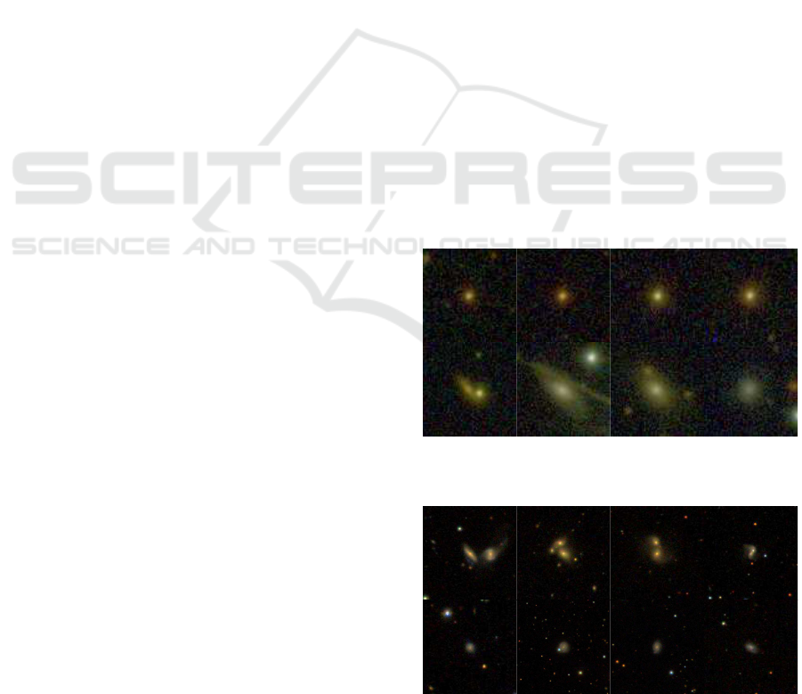
Merging Galaxies (MG): 15766 images divided into

two classes: Merging (5778) and Non-interacting

(9988) galaxies, extracted from the Sloan Digital Sky

Survey (SDSS), Data Release 7 (Abazajian et al.,

2009). This dataset is reasonably large, but the ob-

jects are not as clearly identiﬁable as in the case of

Star/Galaxy classiﬁcation (See Figure 2);

Galaxy Morphology, 2-class (EF-2): 3604 images

divided into two classes: Elliptical (289) and Spiral

(3315) galaxies, extracted from the EFIGI (Baillard

et al., 2011) dataset. This dataset is highly unbalanced

towards images of Spiral galaxies;

Galaxy Morphology, 4-class (EF-4): 4389 images

divided into four classes: Elliptical (289), Spiral

(3315), Lenticular (537) and Irregular (248) galax-

ies, extracted from the EFIGI dataset. The additional

classes makes the classiﬁcation problem harder, since

the objects are not as clearly identiﬁable as in the 2-

class subset (See Figure 3) and classes are highly un-

balanced as well;

Galaxy Morphology, 15-class (EF-15): 4327 im-

ages divided into ﬁfteen classes: Elliptical:-5 (227),

Spiral:0 (196), Spiral:1 (257), Spiral:2 (219), Spi-

ral:3 (517), Spiral:4 (472), Spiral:5 (303), Spiral:6

(448), Spiral:7 (285), Spiral:8 (355), Spiral:9 (263),

Lenticular:-3 (189), Lenticular:-2 (196), Lenticular:-

1 (152), and Irregular:10 (248) galaxies. The num-

bers after the names come from the Hubble Se-

quence (Hubble, 1982), which is a standard taxonomy

used in astronomy for galaxy morphology. This is the

hardest dataset among the evaluated, since it has only

a few hundred observations for each class.

The images from all datasets were reduced to

76x76 pixels, for implementation simplicity, and the

datasets were split into train (80%), validation (10%)

and test sets (10%).

Star

Galaxy

Figure 1: Sample images from the SG dataset.

Merging

Non-interacting

Figure 2: Sample images from the MG dataset.

Deep Learning for Astronomical Object Classiﬁcation: A Case Study

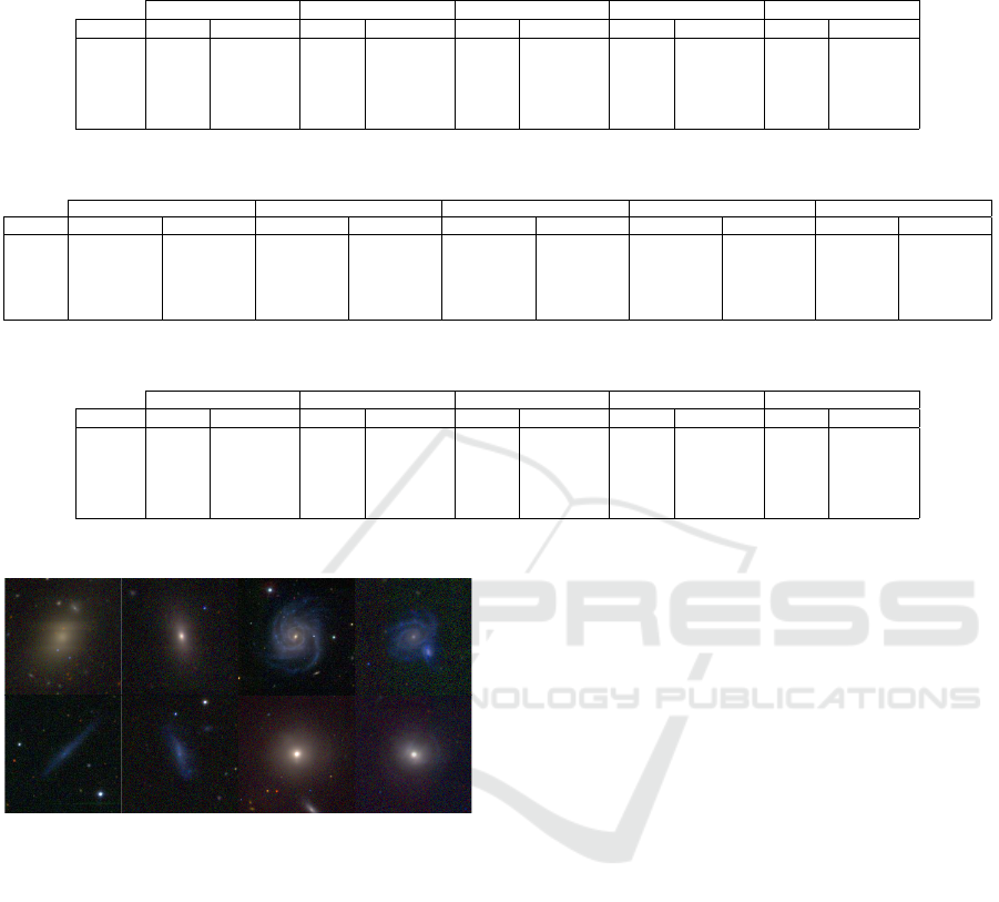
Table 2: Effect of training setup: training from scratch vs. using networks pre-trained with ImageNet on validation accuracy

for all models and all datasets, with λ = 0.1, γ = 0 and the ADAM optimizer. Bold shows best values for each dataset and

model.

DenseNet121 InceptionResNetV2 InceptionV3 ResNext50 VGG16

Dataset scratch pre-trained scratch pre-trained scratch pre-trained scratch pre-trained scratch pre-trained

EF-15 0.329 0.408 0.350 0.373 0.249 0.303 0.282 0.333 0.126 0.459

EF-4 0.782 0.878 0.802 0.869 0.756 0.830 0.772 0.841 0.756 0.878

EF-2 0.958 0.994 0.958 0.989 0.945 0.992 0.952 0.983 0.919 0.994

MG 0.918 0.857 0.875 0.799 0.634 0.784 0.913 0.826 0.634 0.948

SG 0.986 0.961 0.562 0.951 0.782 0.912 0.972 0.951 0.562 0.990

Table 3: Effect of different regularization settings on validation accuracy for all models and all datasets, with optimal values

for λ and γ inside parentheses and the ADAM optimizer. Bold shows best values for each dataset and model.

DenseNet121 InceptionResNetV2 InceptionV3 ResNext50 VGG16

Dataset scratch pre-trained scratch pre-trained scratch pre-trained scratch pre-trained scratch pre-trained

EF-15 0.350 (0,2) 0.408 (0.1,0) 0.350 (0.1,0) 0.373 (0.1,0) 0.249 (0.1,0) 0.303 (0.1,0) 0.301 (0.1,2) 0.333 (0.1,0) 0.422 (0,2) 0.459 (0.1,0)

EF-4 0.835 (0,2) 0.881 (0.1,2) 0.802 (0.1,0) 0.869 (0.1,0) 0.756 (0,0) 0.830 (0.1,0) 0.786 (0.1,2) 0.841 (0.1,0) 0.883 (0,2) 0.883 (0.1,2)

EF-2 0.961 (0,0) 0.994 (0.1,0) 0.962 (0,2) 0.989 (0.1,0) 0.945 (0.1,0) 0.992 (0.1,0) 0.962 (0 ,0) 0.986 (0.1,2) 0.950 (0,2) 0.994 (0.1,0)

MG 0.918 (0.1,0) 0.892 (0,2) 0.901 (0,0) 0.799 (0.1,0) 0.883 (0,2) 0.792 (0 ,0) 0.935 (0 ,0) 0.826 (0.1,0) 0.634 (0,0) 0.952 (0 ,0)

SG 0.989 (0,0) 0.973 (0,2) 0.959 (0,0) 0.952 (0.1,2) 0.914 (0,2) 0.921 (0 ,0) 0.990 (0 ,0) 0.952 (0.1,2) 0.989 (0,0) 0.990 (0.1,2)

Table 4: Effect of different regularization settings: difference between validation accuracy showed in Table 2 and in Table 3.

Bold indicates differences greater than 0.1.

DenseNet121 InceptionResNetV2 InceptionV3 ResNext50 VGG16

Dataset scratch pre-trained scratch pre-trained scratch pre-trained scratch pre-trained scratch pre-trained

EF-15 0.021 0.000 0.000 0.000 0.000 0.000 0.019 0.000 0.296 0.000

EF-4 0.053 0.002 0.000 0.000 0.000 0.000 0.014 0.000 0.127 0.005

EF-2 0.003 0.000 0.004 0.000 0.000 0.000 0.010 0.003 0.031 0.000

MG 0.000 0.036 0.026 0.000 0.250 0.008 0.022 0.000 0.000 0.004

SG 0.003 0.012 0.397 0.002 0.133 0.009 0.019 0.001 0.428 0.000

Elliptical

Spiral

Irregular

Lenticular

Figure 3: Sample images from the EF-2, EF-4 and EF-15

datasets.

3.2 Training Setup

We select ﬁve popular ConvNet architectures for this

experiment, namely VGG16, InceptionV3, Incep-

tionResNetV2, ResNext50 and DenseNet121, as our

starting point. We only use the convolutional part,

i.e., the feature extraction part of each architecture,

and add one 2048-unit dense layer with Glorot weight

initialization (Glorot and Bengio, 2010), constant

bias initialization of 0.01, Leaky ReLU activation

with default settings (Maas et al., 2013), followed

by a Dropout layer (Srivastava et al., 2014) with

0.5 probability of dropping connections, followed

by the softmax layer for classiﬁcation. Given this

setup, we explore the following directions with the

goal of assessing their effect on the overall network

performance:

Training Setup: we train the networks in two distinct

ways:

• From scratch, based on the data alone – we train

the entire network for up to 200 epochs with

Early Stopping, so the training stops automati-

cally if validation loss diverges from training loss

for more than 10 epochs;

• Fine-tuning based on weights from pre-training

on ImageNet – we ﬁrst train the newly added top

layers of the network for 10 epochs, with the con-

volutional part frozen, meaning only the weights

from the top layers are updated, and then we un-

freeze the last 7 layers from the convolutional

part, and train the entire network for up to 200

epochs, with the same Early Stopping setup de-

scribed above and using Stochastic Gradient De-

scent optimizer with learning rate of 0.001 and

momentum of 0.9 (Qian, 1999).

Regularization: in addition to Dropout, we use

the following regularization techniques in the hidden

layer:

• L

regularization (Krogh and Hertz, 1992) (λ): we

set λ ∈ {0.0, 0.1}, with λ = 0.0 meaning no L

regularization;

• Max-norm constraint (Srebro and Shraibman,

VISAPP 2020 - 15th International Conference on Computer Vision Theory and Applications

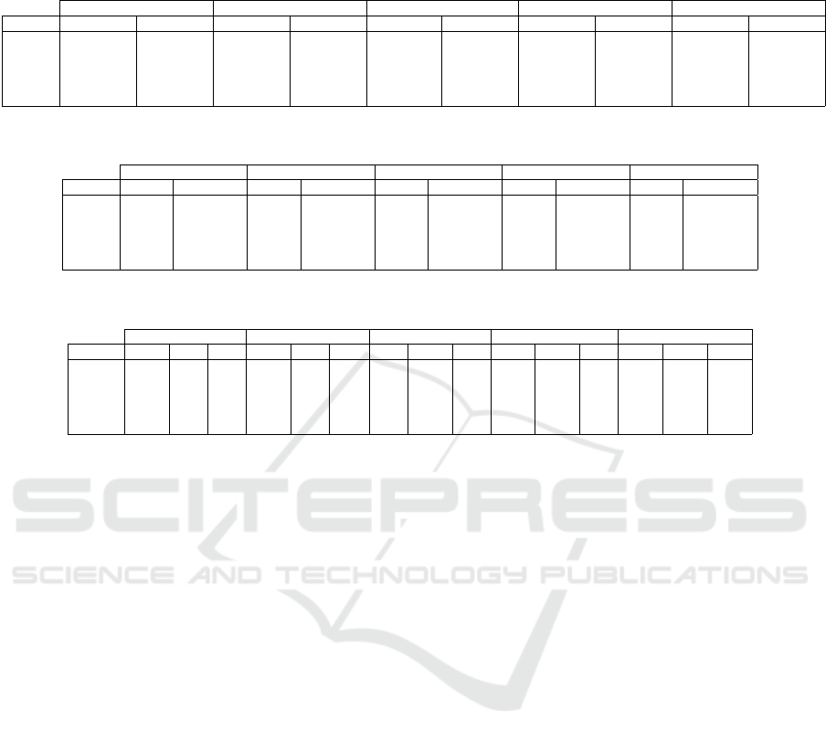
Table 5: Effect of different optimizer settings on validation accuracy for all models and all datasets, with λ = 0.1, γ = 0, with

best optimizer indicated inside parentheses (AD indicates ADAM, RA indicates RADAM, RM indicates RMSprop). Bold

shows best values for each dataset and model.

DenseNet121 InceptionResNetV2 InceptionV3 ResNext50 VGG16

Dataset scratch pre-trained scratch pre-trained scratch pre-trained scratch pre-trained scratch pre-trained

EF-15 0.350 (RA) 0.408 (AD) 0.375 (RA) 0.380 (RM) 0.301 (RA) 0.305 (RA) 0.364 (RA) 0.333 (AD) 0.417 (RA) 0.459 (AD)

EF-4 0.786 (RA) 0.885 (RA) 0.825 (RA) 0.874 (RM) 0.779 (RA) 0.830 (AD) 0.812 (RA) 0.841 (RM) 0.874 (RA) 0.892 (RM)

EF-2 0.958 (RM) 0.994 (RM) 0.961 (RA) 0.989 (RM) 0.945 (AD) 0.992 (RM) 0.952 (AD) 0.985 (RA) 0.965 (RA) 0.994 (RM)

MG 0.918 (AD) 0.858 (RA) 0.923 (RA) 0.799 (AD) 0.827 (RA) 0.784 (AD) 0.913 (AD) 0.827 (RM) 0.634 (RM) 0.949 (RM)

SG 0.992 (RM) 0.965 (RM) 0.975 (RM) 0.952 (RM) 0.782 (AD) 0.912 (AD) 0.990 (RM) 0.952 (RA) 0.562 (RM) 0.990 (RM)

Table 6: Effect of different optimizer settings: difference between validation accuracy showed in Table 2 and in Table 5. Bold

indicates differences greater than 0.1.

DenseNet121 InceptionResNetV2 InceptionV3 ResNext50 VGG16

Dataset scratch pre-trained scratch pre-trained scratch pre-trained scratch pre-trained scratch pre-trained

EF-15 0.021 0.000 0.026 0.007 0.051 0.002 0.082 0.000 0.291 0.000

EF-4 0.005 0.007 0.023 0.005 0.023 0.000 0.039 0.000 0.117 0.014

EF-2 0.000 0.000 0.003 0.000 0.000 0.000 0.000 0.001 0.046 0.000

MG 0.000 0.001 0.047 0.000 0.193 0.000 0.000 0.001 0.000 0.002

SG 0.005 0.005 0.413 0.002 0.000 0.000 0.019 0.001 0.000 0.000

Table 7: Effect of different optimizer settings: average number of epochs until convergence for all optimizers evaluated. AD

indicates ADAM, RA indicates RADAM, RM indicates RMSprop. Bold values indicate the fastest.

DenseNet121 InceptionResNetV2 InceptionV3 ResNext50 VGG16

Dataset RM AD RA RM AD RA RM AD RA RM AD RA RM AD RA

EF-15 2.25 4.5 4.5 7 2.75 4.25 6 2 2.5 8.5 2 3.25 13.75 23 17.5

EF-4 10 4.5 4.5 2.5 2.25 3 1.25 1.5 2 1 1.75 5 1 12.75 28

EF-2 13.25 6 8.25 9.75 1.5 2.5 1.25 5 1.75 3.25 13.25 4.75 1 2.5 12.75

MG 18.5 7.25 6.25 1.75 1.25 1.75 2.5 15.75 2 11.25 50.25 5 9 1 1

SG 27.5 27.5 26 50.75 5 2 3 4.5 3.5 26.5 17.25 26.5 14.5 3.5 8.5

2005) (γ): we set γ ∈ {0, 2}, with γ = 0 meaning

no max-norm constraint.

Optimizers: we use the following adaptive optimiz-

ers, which are popular in Deep Learning literature:

• RMSprop (RM) (Tieleman and Hinton, 2012);

• ADAM (AD) (Kingma and Ba, 2014);

• RADAM (RA) (Liu et al., 2019).

With this combination of hyperparameter values

and training procedures, we expect to achieve a good

compromise between completeness and a reasonable

time frame for executing the full experiment, which is

comprised by 24 training sessions for each model and

dataset, thus yielding a total of 600 runs.

4 RESULTS

We next present the obtained results for each experi-

ment. First, results corresponding to a preset training

conﬁguration is presented and then effects of vary-

ing the hyperparameters are assessed taking this pre-

set conﬁguration as reference.

4.1 Preset Training

We compare the validation accuracy obtained on each

dataset with models trained from scratch and with

pre-trained models plus ﬁne-tuning. For this assess-

ment, among all results, we selected the ones from the

experiments that used λ = 0.1, γ = 0 and the ADAM

optimizer, as these are commonly used preset values

for those parameters. We see in Table 2 that, with a

few exceptions for the larger datasets (SG and MG),

using pre-training yields models with higher valida-

tion accuracy for all studied datasets, in some cases

by a large margin.

4.2 Regularization

We train all models with different regularization set-

tings to assess their effect depending on training

setup (from scratch or pre-trained), network architec-

ture/model, and dataset. In Table 3 we see the vali-

dation accuracy obtained with the best regularization

settings, for all models and datasets, and in Table 4

we see the difference between results obtained with a

ﬁxed preset (See Table 2) and the optimal. In most

cases the difference is very small, but in a few cases

ﬁnding the optimal regularization settings made a sig-

niﬁcant difference. Another interesting ﬁnding is that

the signiﬁcant improvements were achieved only with

training from scratch, which indicates that the pre-

trained network is less sensitive to those settings.

Deep Learning for Astronomical Object Classiﬁcation: A Case Study

Table 8: Best models overall: Accuracy achieved for each dataset and model with optimal settings, as described in Table 10.

Bold shows best values for each dataset and model.

DenseNet121 InceptionResNetV2 InceptionV3 ResNext50 VGG16

Dataset scratch pre-trained scratch pre-trained scratch pre-trained scratch pre-trained scratch pre-trained

EF-15 0.350 0.408 0.392 0.389 0.301 0.310 0.364 0.338 0.436 0.476

EF-4 0.835 0.885 0.835 0.874 0.782 0.830 0.812 0.841 0.883 0.903

EF-2 0.962 0.994 0.969 0.989 0.959 0.992 0.962 0.986 0.994 0.994

MG 0.923 0.894 0.929 0.803 0.896 0.797 0.935 0.827 0.941 0.952

SG 0.992 0.973 0.975 0.952 0.914 0.921 0.992 0.952 0.992 0.991

Table 9: Best models overall: difference between validation accuracy showed in Table 2 and in Table 8. Bold indicates

differences greater than 0.1.

DenseNet121 InceptionResNetV2 InceptionV3 ResNext50 VGG16

Dataset scratch pre-trained scratch pre-trained scratch pre-trained scratch pre-trained scratch pre-trained

EF-15 0.021 0.000 0.042 0.016 0.051 0.007 0.082 0.005 0.310 0.016

EF-4 0.053 0.007 0.032 0.005 0.025 0.000 0.039 0.000 0.127 0.025

EF-2 0.004 0.000 0.011 0.000 0.014 0.000 0.010 0.003 0.076 0.000

MG 0.005 0.038 0.054 0.004 0.263 0.013 0.022 0.001 0.308 0.004

SG 0.005 0.012 0.413 0.002 0.133 0.010 0.020 0.001 0.430 0.001

Table 10: Best models overall: Optimal settings (λ, γ and optimizer) used for achieving results in Table 8.

DenseNet121 InceptionV3 VGG16 ResNext50 VGG16

Dataset scratch pre-trained scratch pre-trained scratch pre-trained scratch pre-trained scratch pre-trained

EF-15 0.0, 2, AD 0.1, 0, AD 0.1, 2, RA 0.1, 2, RA 0.1, 0, RA 0.1, 2, RM 0.1, 0, RA 0.1, 2, RM 0.0, 0, RA 0.1, 2, RA

EF-4 0.0, 2, AD 0.1, 0, RA 0.0, 2, RA 0.1, 0, RM 0.0, 0, RA 0.1, 0, AD 0.1, 0, RA 0.0, 0, RM 0.0, 2, AD 0.0, 0, RM

EF-2 0.0, 2, RM 0.1, 0, RM 0.0, 2, RA 0.1, 0, RM 0.1, 2, RA 0.1, 0, RM 0.0, 0, AD 0.1, 2, AD 0.0, 2, RA 0.0, 2, RM

MG 0.0, 2, RA 0.0, 2, RA 0.0, 0, RA 0.1, 2, RM 0.1, 2, RA 0.0, 2, RA 0.0, 0, AD 0.1, 0, RM 0.0, 2, RM 0.0, 0, AD

SG 0.1, 0, RM 0.0, 2, AD 0.1, 0, RM 0.1, 0, RM 0.0, 2, AD 0.0, 2, RM 0.1, 2, RM 0.1, 2, AD 0.0, 2, RA 0.1, 2, RA

4.3 Optimizers

We experiment with different optimizers to assess the

effect they play on accuracy and convergence speed.

In Table 5 we see the validation accuracy obtained

with the best optimizer for each training setup, model

and dataset, and in Table 6 we see the difference be-

tween results obtained with a ﬁxed preset (Table 2)

and the optimal. In this case, the difference is less

noticeable than in the case of regularization settings,

with only a few combinations showing signiﬁcant im-

provement. As in the case of regularization, the sig-

niﬁcant improvement, where exists, is achieved only

when training from scratch.

Regarding convergence speed, in Table 7, we see

that in most cases, there is an association between the

fastest optimizer for a certain architecture, regardless

of the dataset. This may indicate that some optimizers

are more suitable to certain types of models, accord-

ing the certain intrinsic characteristics, such as num-

ber of parameters, existence of residual connections,

and so on.

4.4 Best Models Overall

Finally, by combining the best optimizer settings with

the best regularization settings, we get to the best

models overall for each dataset, as seen in Tables 8

and 9. We see that signiﬁcant improvement can be

achieved by ﬁnding the right combination of model,

optimizer and regularization settings for a speciﬁc

problem, however, ﬁnding those optimal settings can

be very time-consuming. It seems also that there

are only few cases where performance is signiﬁcantly

better than the preset case. Table 10 shows the opti-

mal settings for each model and dataset.

5 DISCUSSION

We next summarize the obtained insights, as follows.

Which of the ﬁve models is more appropriate to which

classiﬁcation problem?

In Tables 11 and 12 we see the best models for

each dataset, ranked by accuracy, in both training

setups. We notice that the VGG16 architecture

yielded the best performance for all datasets, on both

training setups and in some cases by a large margin.

Since astronomy images are quite simpler than the

ones from ImageNet, usually with an object in the

center surrounded by a dark background, we believe

that VGG16’s much larger number of parameters

might have been instrumental in helping the network

discriminate images that vary little per class. When

looking at the second best model, we see different

trends depending on the training setup: when trained

from scratch, InceptionResNetV2 produced the best

results for the smaller datasets (EF-2, EF-4 and

EF-15), while the larger datasets (SG and MG)

achieved the best results with ResNext50; when

pre-trained on ImageNet, DenseNet121 is the overall

second-best. We also see that InceptionV3 was the

VISAPP 2020 - 15th International Conference on Computer Vision Theory and Applications

Table 11: Best models for each dataset, ranked by accuracy, trained from scratch.

EF-15 EF-2 EF-4 MG SG

VGG16 (0.436) VGG16 (0.994) VGG16 (0.883) VGG16 (0.941) VGG16 (0.992)

InceptionResNetV2 (0.392) InceptionResNetV2 (0.969) InceptionResNetV2 (0.835) ResNext50 (0.935) ResNext50 (0.992)

ResNext50 (0.364) ResNext50 (0.959) DenseNet121 (0.835) InceptionResNetV2 (0.929) DenseNet121 (0.992)

DenseNet121 (0.350) DenseNet121 (0.962) ResNext50 (0.812) DenseNet121 (0.923) InceptionResNetV2 (0.975)

InceptionV3 (0.301) InceptionV3 (0.959) InceptionV3 (0.782) InceptionV3 (0.896) InceptionV3 (0.914)

Table 12: Best models for each dataset, ranked by accuracy, pre-trained on ImageNet.

EF-15 EF-2 EF-4 MG SG

VGG16 (0.476) VGG16 (0.994) VGG16 (0.903) VGG16 (0.991) VGG16 (0.991)

DenseNet121 (0.408) DenseNet121 (0.994) DenseNet121 (0.885) DenseNet121 (0.894) DenseNet121 (0.973)

InceptionResNetV2 (0.389) InceptionV3 (0.992) InceptionResNetV2 (0.874) ResNext50 (0.827) ResNext50 (0.952)

ResNext50 (0.338) InceptionResNetV2 (0.989) ResNext50 (0.841) InceptionResNetV2 (0.803) InceptionResNetV2 (0.952)

InceptionV3 (0.310) ResNext50 (0.986) InceptionV3 (0.830) InceptionV3 (0.797) InceptionV3 (0.921)

worse-performing model on almost every case. In

summary, we see a trend emerge, with models con-

taining many parameters performing best, followed

by models with residual connections, followed by

models without residual connections. Since models

with residual connections are faster to train and run

inference on than VGG-style models, a user could

trade-off some accuracy for speed if required.

Which set of hyperparameters is the best for each

model and for each problem?

In Table 10 we see that regularization settings are

highly dependent on the model and training setup, and

less dependent on the data. For example, when trained

from scratch, DenseNet121 achieves top accuracy in

most cases with λ = 0.0 and γ = 2, whereas when pre-

trained on ImageNet, it achieves top accuracy in most

cases with λ = 0.1 and γ = 2. InceptionV3 presents

a similar pattern, while VGG16 works best in most

cases with λ = 0.0 and γ = 2, regardless of training

setup. In the speciﬁc case of VGG16, we expected

a model as large as VGG16 to require stronger regu-

larization, but we found that max-norm and dropout

works best, which corroborates the results of (Srivas-

tava et al., 2014). Regarding optimizer, the pattern

is less clear, with some models working best with a

single optimizer depending on the training setup, like

InceptionV3 with RADAM (from scratch) and RM-

Sprop (pre-trained). The RADAM optimizer, which

is fairly new development in the area, performed well

if we look at how many times it appeared as the best

choice, but it does not seem to have a very big im-

provement over ADAM and RMSprop.

When is ImageNet pre-training beneﬁcial?

In all cases except one (which is an almost-tie, for

the SG dataset), the highest accuracy was achieved

by using models pre-trained on ImageNet, with a ﬁve

percentage-point-improvement for the dataset MG.

We see this as conﬁrmation that models pre-trained on

ImageNet can be used as generic feature extractors for

images in very different domains, such as astronomy,

with little effort.

How do the number of classes and observations affect

model performance?

We see that VGG16 achieved almost perfect

scores for the larger datasets (SG and MG) on both

training setups. This was expected, since the datasets

are reasonably large and have only two classes each.

The datasets EF-2 and EF-4, despite being quite small

for ConvNets, also worked very well with VGG16,

which might be due to the fact that the images are of

higher quality when compared to the others, and that

they only have a few classes as well. However, in

the case of EF-15, even the best model achieves accu-

racy below 50%. In this case, we believe the higher

number of classes along with the small number of ob-

servations per class played a central role.

6 CONCLUSION

We presented an in-depth study aimed at evaluating

different ConvNet architectures for different astro-

nomical object classiﬁcation problems. We presented

results for ﬁve popular architectures and ﬁve datasets

representing three different problems in astronomy.

We showed how training setup, optimizer and reg-

ularization settings affect the accuracy for different

architectures and datasets, and we conclude that for

all problems studied here, VGG-style architectures

pre-trained on ImageNet perform the best, even with

smaller datasets, followed by models with residual

connections such as DenseNet, InceptionResNetV2

and ResNext.

We plan to extend this work in the direction of ex-

ploring different feature extraction techniques, in par-

ticular, by ﬁnding ways of leveraging the enormous

amount of unlabeled data which exists in astronomy.

All experiments were executed on a computer

with a quad-core Intel E3-1240v6 running at 3.7 GHz,

64 GB of RAM and an NVidia GTX 1080 Ti GPU

with 11 GB of Video RAM.

Deep Learning for Astronomical Object Classiﬁcation: A Case Study

ACKNOWLEDGMENTS

This study was ﬁnanced in part by FAPESP

(2015/22308-2, 2017/25835-9 and 2018/25671-9)

and the Coordenac¸

ao de Aperfeic¸oamento de Pessoal

de N

ıvel Superior - Brasil (CAPES) - Finance Code

001.

REFERENCES

Abazajian, K. N. et al. (2009). The Seventh Data Release

of the Sloan Digital Sky Survey. The Astrophysical

Journal Supplement Series, 182(2):543–558.

Ackermann, S., Schawinski, K., Zhang, C., Weigel, A. K.,

and Turp, M. D. (2018). Using transfer learning to

detect galaxy mergers. Monthly Notices of the Royal

Astronomical Society, 479(1):415–425.

Aniyan, A. and Thorat, K. (2017). Classifying radio galax-

ies with the convolutional neural network. The Astro-

physical Journal Supplement Series, 230(2):20.

Baillard, A., Bertin, E., De Lapparent, V., Fouqu

e, P.,

Arnouts, S., Mellier, Y., Pell

o, R., Leborgne, J.-F.,

Prugniel, P., Makarov, D., et al. (2011). The EFIGI

catalogue of 4458 nearby galaxies with detailed mor-

phology. Astronomy & Astrophysics, 532:A74.

Ball, N. M. and Brunner, R. J. (2010). Data mining and

machine learning in astronomy. International Journal

of Modern Physics D, 19(07):1049–1106.

Bengio, Y. (2012). Deep learning of representations for

unsupervised and transfer learning. In Proc. ICML,

pages 17–36.

Bertin, E. (1994). Classiﬁcation of astronomical images

with a neural network. Astrophysics and Space Sci-

ence, 217(1-2):49–51.

Bertin, E. and Arnouts, S. (1996). Sextractor: Software for

source extraction. Astronomy and Astrophysics Sup-

plement Series, 117(2):393–404.

Deng, J., Dong, W., Socher, R., Li, L.-J., Li, K., and Fei-

Fei, L. (2009). Imagenet: A large-scale hierarchical

image database. In Proc. CVPR, pages 248–255.

Dieleman, S., Willett, K. W., and Dambre, J. (2015).

Rotation-invariant convolutional neural networks for

galaxy morphology prediction. Monthly notices of the

Royal Astronomical Society, 450(2):1441–1459.

Ferrari, F., de Carvalho, R. R., and Trevisan, M. (2015).

Morfometryka – a new way of establishing morpho-

logical classiﬁcation of galaxies. The Astrophysical

Journal, 814(1):55.

Gauci, A., Adami, K. Z., and Abela, J. (2010). Machine

Learning for Galaxy Morphology Classiﬁcation.

Glorot, X. and Bengio, Y. (2010). Understanding the dif-

ﬁculty of training deep feedforward neural networks.

In Proc. AISTATS, pages 249–256.

He, K., Zhang, X., Ren, S., and Sun, J. (2016). Deep resid-

ual learning for image recognition. Proc. CVPR.

Huang, G., Liu, Z., Maaten, L. v. d., and Weinberger, K. Q.

(2017). Densely connected convolutional networks.

Proc. CVPR.

Hubble, E. P. (1982). The realm of the nebulae, volume 25.

Yale University Press.

Ivezi

Z., Connolly, A. J., VanderPlas, J. T., and Gray, A.

(2014). Statistics, Data Mining, and Machine Learn-

ing in Astronomy: A Practical Python Guide for the

Analysis of Survey Data. Princeton University Press.

Kim, E. J. and Brunner, R. J. (2016). Star-galaxy clas-

siﬁcation using deep convolutional neural networks.

Monthly Notices of the Royal Astronomical Society,

page 2672.

Kingma, D. and Ba, J. (2014). Adam: A method for

stochastic optimization. arXiv:1412.6980.

Krizhevsky, A., Sutskever, I., and Hinton, G. E. (2012). Im-

agenet classiﬁcation with deep convolutional neural

networks. In Advances in Neural Information Pro-

cessing Systems, pages 1097–1105.

Krogh, A. and Hertz, J. A. (1992). A simple weight de-

cay can improve generalization. In Proc. NIPS, pages

950–957.

Lintott, C. J., Schawinski, K., Slosar, A., Land, K., Bam-

ford, S., Thomas, D., Raddick, M. J., Nichol, R. C.,

Szalay, A., Andreescu, D., Murray, P., and Vanden-

berg, J. (2008). Galaxy Zoo: morphologies derived

from visual inspection of galaxies from the Sloan Dig-

ital Sky Survey. Monthly Notices of the Royal Astro-

nomical Society, 389(3):1179–1189.

Liu, L., Jiang, H., He, P., Chen, W., Liu, X., Gao, J., and

Han, J. (2019). On the variance of the adaptive learn-

ing rate and beyond.

Maas, A. L., Hannun, A. Y., and Ng, A. Y. (2013). Rec-

tiﬁer nonlinearities improve neural network acoustic

models. In Proc. ICML, volume 30, page 3.

Moore, J. A., Pimbblet, K. A., and Drinkwater, M. J.

(2006). Mathematical morphology: Star/galaxy dif-

ferentiation & galaxy morphology classiﬁcation. Pub-

lications of the Astronomical Society of Australia,

23(04):135146.

Odewahn, S. (1995). Automated classiﬁcation of astronom-

ical images. Publications of the Astronomical Society

of the Paciﬁc, 107(714):770.

Oliveira, C. M., Ribeiro, T., Schoenell, W., Kanaan, A.,

Overzier, R. A., Molino, A., Sampedro, L., Coelho,

P., Barbosa, C. E., Cortesi, A., Costa-Duarte, M. V.,

Herpich, F. R., et al. (2019). The Southern Photo-

metric Local Universe Survey (S-PLUS): improved

SEDs, morphologies and redshifts with 12 optical ﬁl-

ters. arXiv:1907.01567.

Pan, S. J. and Yang, Q. (2009). A survey on transfer learn-

ing. Proc. TKDE, 22(10):1345–1359.

Qian, N. (1999). On the momentum term in gradi-

ent descent learning algorithms. Neural networks,

12(1):145–151.

Russakovsky, O., Deng, J., Su, H., Krause, J., Satheesh,

S., Ma, S., Huang, Z., Karpathy, A., Khosla, A.,

Bernstein, M., Berg, A. C., and Fei-Fei, L. (2015).

ImageNet Large Scale Visual Recognition Challenge.

International Journal of Computer Vision (IJCV),

115(3):211–252.

Sanchez, H. et al. (2018). Transfer learning for galaxy mor-

VISAPP 2020 - 15th International Conference on Computer Vision Theory and Applications

phology from one survey to another. Monthly Notices

of the Royal Astronomical Society, 484(1):93–100.

Simonyan, K. and Zisserman, A. (2014). Very deep convo-

lutional networks for large-scale image recognition.

Srebro, N. and Shraibman, A. (2005). Rank, trace-norm and

max-norm. In Proc. COLT, pages 545–560. Springer.

Srivastava, N., Hinton, G., Krizhevsky, A., Sutskever, I.,

and Salakhutdinov, R. (2014). Dropout: a simple way

to prevent neural networks from overﬁtting. JMLR,

15(1):1929–1958.

Szegedy, C., Ioffe, S., Vanhoucke, V., and Alemi, A.

(2016a). Inception-v4, inception-resnet and the im-

pact of residual connections on learning.

Szegedy, C., Vanhoucke, V., Ioffe, S., Shlens, J., and Wojna,

Z. (2016b). Rethinking the inception architecture for

computer vision. Proc. CVPR.

Tieleman, T. and Hinton, G. (2012). Rmsprop: Divide

the gradient by a running average of its recent magni-

tude. coursera: Neural networks for machine learning.

Technical report, page 31.

Xie, S., Girshick, R., Doll

ar, P., Tu, Z., and He, K. (2017).

Aggregated residual transformations for deep neural

networks. In Proc. CVPR, pages 1492–1500. IEEE.

Deep Learning for Astronomical Object Classiﬁcation: A Case Study