
Optimization of a Sequential Decision Making Problem for a Rare
Disease Diagnostic Application
R
´
emi Besson
1
, Erwan Le Pennec
1,4
, Emmanuel Spaggiari
2
, Antoine Neuraz
2
, Julien Stirnemann
2
and St
´
ephanie Allassonni
`
ere
3
1
CMAP,
´
Ecole Polytechnique, Route de Saclay, 91128 Palaiseau, France
2
Necker-Enfants Malades Hospital, Paris-Descartes University, 149 Rue De S
`
evres, 75015 Paris, France
3
School of Medicine, Paris-Descartes University, 15 Rue de l’
´
Ecole de M
´
edecine, 75006 Paris, France
4
XPop, Inria Saclay, 91120 Palaiseau, France
Keywords:
Symptom Checker, Stochastic Shortest Path, Decision Tree Optimization, Planning in High-dimension.
Abstract:
In this work, we propose a new optimization formulation for a sequential decision making problem for a rare
disease diagnostic application. We aim to minimize the number of medical tests necessary to achieve a state
where the uncertainty regarding the patient’s disease is less than a predetermined threshold. In doing so, we
take into account the need in many medical applications, to avoid as much as possible, any misdiagnosis. To
solve this optimization task, we investigate several reinforcement learning algorithms and make them operable
in our high-dimensional setting: the strategies learned are much more efficient than classical greedy strategies.
1 INTRODUCTION
Motivation. The development of a decision support
tool for medical diagnosis has long been an objec-
tive. In the 1980s, researchers were already trying
to develop an algorithm that would allow them to find
the patient’s disease by sequentially asking questions
about the relevant symptoms.
Recent works aim to apply the breakthrough of
reinforcement learning (RL) to learn good diagnos-
tic strategy, see for example (Chen et al., 2019). We
present in this work our contributions to this objective
of adapting the new progress of machine learning for
the optimization of symptom checkers.
We are particularly interested in the field of rare
diseases where such a tool is particularly desirable.
Indeed, no doctor has the encyclopedic knowledge to
take into account all diagnoses, because rare diseases
are numerous and each of them will be observed only
a very small number of times or never in the doc-
tor’s career. As a result, rare diseases are often under-
diagnosed or diagnosed late after medical wandering.
A symptom checker for the prenatal diagnosis of
rare diseases by fetal ultrasound would be even more
useful. Indeed, in this particular case, the patient can
not describe the symptoms himself and the physician
has to check several anatomical regions looking for
abnormalities that can be hard to detect.
We aim to help the practitioner make the diagnosis
with a high probability while minimizing the average
number of symptoms to be checked. To do this, we
design an algorithm that proposes the most promising
symptoms to be checked at each stage of the medi-
cal examination and provides the probability of each
possible disease. Eventually, our algorithm must be
operable and interpretable online at the bedside.
Note that this article only presents the optimiza-
tion task associated with recommending the next
symptoms to be checked. Several other modules are
needed to build the final decision support tool. We
detail some of them in (Besson, 2019), including the
one that builds the environment model and another
that deals with the granularity of symptoms.
Available Data and Some Dimensions. The data
is structured as a list of diseases with their estimated
prevalence in the whole population and a list of symp-
toms for each disease. We will call them associated or
typical symptoms. We also have an estimation of the
probability of the symptom given the disease. We de-
note B
i
the binary random variable (r.v) associated to
the presence/absence of symptom of type i.
All this information, that we will refer to as expert
data, has been provided by physicians of Necker hos-
Besson, R., Pennec, E., Spaggiari, E., Neuraz, A., Stirnemann, J. and Allassonnière, S.
Optimization of a Sequential Decision Making Problem for a Rare Disease Diagnostic Application.
DOI: 10.5220/0008938804750482
In Proceedings of the 12th International Conference on Agents and Artificial Intelligence (ICAART 2020) - Volume 2, pages 475-482
ISBN: 978-989-758-395-7; ISSN: 2184-433X
Copyright
c
2022 by SCITEPRESS – Science and Technology Publications, Lda. All rights reserved
475

pital based on the available literature. We map all the
symptoms found in the literature to the Human Phe-
notype Ontology (HPO) (K
¨
ohler and al., 2017). HPO
is a recent work which provides a standardized vocab-
ulary of phenotypic abnormalities encountered in hu-
man disease. We use it to harmonize the terminology.
We could then combine our list of symptoms per dis-
ease and map it to OrphaData
1
. OrphaData is useful
to fill the missing data on prevalence of symptoms in
the diseases. We restrict our analyses to the subset of
symptoms that can be detected using fetal ultrasound.
We assume, in this work, that we know the joint
distribution of the typical symptoms given the dis-
ease. This issue is addressed in (Besson et al.,
2019). We proposed a method to mix expert data
(the marginals and some additional constraints as for
example censored combinations) with clinical data
which is collected as the algorithm is used. We there-
fore focus in this work on the planning task since we
assume the environment model to be known and fixed.
Currently, our database references 81 diseases and
220 symptoms. We make the assumption that a pa-
tient presents only one disease at a time which is a
reasonable hypothesis in the rare disease framework.
Main Contributions. The main contributions of
this work are the following: we propose a novel no-
tion of what should be a good symptom checker, tak-
ing into account the need in medicine to have a high
level of confidence in the diagnosis made. This led us
to formulate the task of optimizing symptom check-
ers as a stochastic shortest path problem. We also de-
tail in section 4.4 a new algorithm that we call DQN-
MC-Bootstrap inspired by DQN from (Mnih et al.,
2013). We have drastically reduced the computing
power needed to solve our problem by partitioning
the state space and appropriately using the connec-
tions between the subtasks with DQN-MC-Bootstrap.
2 RELATED WORKS
Shortest Path Algorithms. A
?
is a classic algorithm
which finds the minimum cost path between a start
node and a final node through a deterministic graph
(Hart et al., 1968). (Zubek and Dietterich, 2005) pro-
posed an algorithm inspired of a variant of A
?
for
the optimization of the medical diagnostic procedure.
Nevertheless such an approach is not tractable in a
high-dimensional graph since its assume the possibil-
ity to store the whole tree of the paths investigated.
1
Orphanet. INSERM 1997. An online rare disease and
orphan drug data base. http://www.orpha.net. Accessed
[02/10/2018]
Some improvements using less memory have been
proposed as IDA
?
(Korf, 1985). However, this algo-
rithm does not exactly match our problem. We are
not looking for a single shortest path in a deterministic
graph, but rather to find for each node of the graph the
shortest path to the objective states. Indeed, since we
allow the doctor to answer a different question than
the one we propose, we want to have a good solution
even in a part of the tree that is not the optimal path. In
this sense, we cannot avoid using some form of policy
parameterization in the hope that a good solution on
the optimized part of the tree will have learned a good
enough representation of the state to be good on the
unvisited part of the tree.
Disease Diagnostic Task using RL Algorithms.
Recent works (Chen et al., 2019), (Peng et al., 2018),
(Tang et al., 2016) focus on this problem of optimiz-
ing symptom checkers using RL algorithms. Never-
theless our approach is fairly different to these previ-
ous works. They formulated their optimization prob-
lem as a trade-off between asking less questions and
making the right diagnosis while we formulate it as
the task of reaching as quick as possible, on average,
a pre-determined high degree of certainty about the
patient disease. In our case, the parameter to be tuned
is the degree of certainty we want at the end of the
examination: we should stop when the entropy of the
disease falls below this threshold ε. The smaller the
ε the more symptoms our algorithm will need before
considering that the game ends.
(Tang et al., 2016) makes use of a discounted fac-
tor γ ∈ [0,1[ in their reward signal design. The reward
associated to each question is zero until possessing
a diagnosis (which is an additional possible action)
where the reward is equal to γ
q
(if the guess was cor-
rect, 0 otherwise), q being the number of questions
that have been inquired before possessing the diagno-
sis. In this context γ makes the compromise between
asking fewer question and making the right diagnosis.
The smaller γ, the more likely the algorithm is to make
a wrong diagnosis by trying to ask fewer questions.
3 A MARKOV DECISION
PROCESS FRAMEWORK
3.1 The Optimization Problem
Modelization. We formulate our sequential deci-
sion making problem using the Markov Decision Pro-
cess (MDP) framework. For the state space S, we use
ICAART 2020 - 12th International Conference on Agents and Artificial Intelligence
476

the ternary base encoding 1 if the considered symp-
tom is present, 0 if it is absent, 2 if non observed yet:
S =
(2,...,2),(1,2,..., 2),. ..,(0,.. ., 0)
.
An element s ∈ S is a vector of length 220 (the
number of possible symptoms), it sums up our state
of knowledge about the patient’s condition: the i-th
element of s encode information about the symptom
whose identifier is i.
Concerning the action space A, we write A =
a
1
,...,a
220
. An action is a symptom that we sug-
gest to the obstetrician to look for, more specifically
a
j
is the action to suggest to check symptom j.
Our environment dynamic is by construc-
tion Markovian in the sense that P[s
t+1
|
a
t
,s
t
,a
t−1
,s
t−1
,...a
0
,s
0
] = P[s
t+1
| a
t
,s
t
] where
a
t
is the action taken at time t.
Diagnostic Policy. We aim to learn a diagnostic
policy that associates each state of knowledge (list of
presence/absence of symptoms) with an action to take
(a symptom to check), π : S → A. What should be a
good diagnostic policy? Many medical applications
consider a trade-off between the cost of performing
more medical tests (measuring it in time or money)
and the cost of a misdiagnosis (Tang et al., 2016),
(Zubek and Dietterich, 2005).
However in our case the cost of performing more
medical tests (i.e to check more possible symptoms)
is negligible against the potential cost of a misdiagno-
sis. In theory, the obstetrician have to check all possi-
ble symptoms to ensure the fetus does not present any
disease. Therefore we do not take the risk of a misdi-
agnosis by trying to ask fewer questions. However if
the physician observes a sufficient amount of symp-
toms he can stop the ultrasound examination and per-
form additional tests, like an amniocentesis, to con-
firm his hypotheses.
This is why we can label some states as terminal:
they satisfy the condition that the entropy of the r.v
disease is so low that we have no doubt on the diag-
nosis. Our goal is to minimize the average number of
inquiries before reaching a terminal state:
π
?
= argmin
π
E
P
I
s
0
,π
, (1)
where s
0
= (2,..., 2) is the initial state, P the law of
the environment currently used, π the diagnostic pol-
icy, and I is the random number of inquiries before
reaching a terminal states, i.e:
I = inf{t | H(D | S
t
) ≤ ε} (2)
where H(D | S
t
) =
∑
s
t
P[S
t
= s
t
]H(D | S
t
= s
t
) is the
entropy of the r.v disease D given what we know at
time t: S
t
. We should think s
t
as a realization of S
t
.
Note that we are not ensured that for all t we had
H(D | s
t+1
) ≤ H(D | s
t
). Nevertheless this inequality
holds when taking the average H(D | S
t+1
) ≤ H(D |
S
t
), see theorem 2.6.5 of (Cover and Thomas, 2006),
”information can’t hurt”. Then, when we consider
that entropy is sufficiently low and that we can stop
and propose a diagnosis, we know that on average, the
uncertainty about the patient’s disease would not have
increased if we had continued checking symptoms.
Setting a reward function as follow, ∀s
t
,a
t
:
r
t+1
:= r(s
t
,a
t
) = −1, (3)
we can write (1) as a classical episodic reinforcement
learning problem (Sutton and Barto, 2018):
π
?
= argmax
π
E
P
"
I
∑
t=1
r
t
s
0
,π
#
. (4)
In RL such a reward design is called action-
penalty representation, since the agent is penalized for
every action executed. It is notably a classic way to
model shortest path problems.
The Use of the Environment Model. Theoretically
the environment model that we have at our disposal,
the joint distribution of the combination of symptoms
given the disease, provides us with a transition model.
Nevertheless, in practice, we do not use directly
the model. It is indeed not possible to store the tran-
sition matrix for dimensional reasons. That is why
our only alternative to solve the optimization problem
(4) is to simulate games by recalculating the transition
probabilities on the fly. Moreover, the incremental na-
ture of the states implies that the cost for simulating a
game from the start s
0
to a certain state s
t
is approxi-
mately the same than the cost to do an unique transi-
tion from state s
t−1
to s
t
. That is why our environment
model should be looked in practice as a simulator of
games starting from state s
0
to s
I
.
Finally, note that a subtlety of our stopping crite-
rion (2) is that it requires us to compute the probabil-
ities of the diseases given the symptoms combination
of the current state at each step of the medical exam-
ination. Indeed for dimensional reasons we can not
store the set of goal states and have to check at each
step if we can stop and possess a diagnostic or not.
Note that (4) is more a planning problem than a
RL one since we assume to know the environment law
P and aim to solve the MDP associated. Nevertheless,
since the dimension of our problem is high, we solve
the MDP by sampling trajectories and then treating
the environment model as a simulator which blurs the
boundaries between RL and planning.
Optimization of a Sequential Decision Making Problem for a Rare Disease Diagnostic Application
477

3.2 Decomposition of the State Space
Our full model is of very high dimension: we have
220 different symptoms and then theoretically 3
220
≈
10
104
different states. Thus a tabular dynamic pro-
gramming approach (section 4.1) is impossible. Ac-
cording to our experiments, a classical Deep-Q learn-
ing is also not numerically tractable (section 4.2).
In order to break the dimension, we capitalize
first on the fact that the physicians use our algorithm
mainly after seeing a first symptom. In such case, we
make the assumption that this initial symptom is typ-
ical. It might be possible to have a disease which also
presents a non-typical symptom but this happens with
a low probability. Anyway, in this case, we would end
up with a high entropy and no disease identification.
This leads to switch to another strategy. With such
an assumption the dimension drops significantly since
we now only consider diseases for which this initial
symptom is typical, the only relevant symptoms are
the one which are typical of these remaining diseases.
Therefore we created 220 tasks T
i
to solve. We
denote B
i
= (B
i
1
,...,B
i
k
) the set of symptoms related
with the symptom i, i.e this is the set of symptoms
which are still relevant to check after observing the
presence of symptom i. For all i, we start from state
s
(i)
which is the state of length |B
i
| with the presence
of symptom B
i
and no other information on the others
symptoms, and we aim to solve:
π
?
(i)
= argmax
π
E
P
"
I
∑
t=1
r
t
| s
(i)
,π
#
. (T
i
)
In RL, there exist several ways to solve a prob-
lem like (T
i
). If the dimension is small enough it is
possible to find the optimal solution explicitly using
a dynamic programming algorithm (see section 4.1).
If the number of states is too high we have to param-
eterize the policy, section 4.5, or to parameterize the
Q-values, section 4.2. We have investigated both ap-
proaches to solve our problem.
4 A VALUE-BASED APPROACH
4.1 Look-up Table Algorithm
We recall that the Q-values are defined as Q
π
(s,a) =
E
∑
I
t
0
=t
r
t
0
| s
t
= s,a
t
= a,π
. This is the expecting
amount of reward when starting from state s, taking
action a and then following the policy π. The optimal
Q-values, are defined as Q
?
(s,a) = max
π
Q
π
(s,a) and
satisfy the following Bellman optimality equation:
Q
?
(s,a) = r(s,a) +
∑
s
0
P[s
0
| s,a] max
a
0
∈A
Q
?
(s
0
,a
0
)
The optimal policy π
?
, is directly derived from
Q
?
: π
?
(s) = arg max
a
Q
?
(s,a). Therefore we ”only”
need to evaluate Q
?
(s,a), ∀s,a. This can be done by
a value-iteration algorithm which uses the Bellman
equation as an iterative update:
Q
?
k+1
(s,a) ← r(s,a) +
∑
s
0
P[s
0
| s,a] max
a
0
∈A
Q
?
k
(s
0
,a
0
).
It is known, see (Sutton and Barto, 2018), that
Q
k
→ Q
?
when k → ∞. The main limitation of this al-
gorithm is to require the storage of all Q-values which
is of course not possible when the size of the state
space is large.
4.2 Q-learning with Function
Approximation
To cope with the high dimensionality of the state
space, the idea is to parameterize the Q-values by a
neural network: Q(s,a) ≈ Q
w
(s,a) called Q-network.
It takes as input the state and output the different Q-
values. The heuristic for training such a Q-network
is to simulate transitions (s
t
,a
t
,r
t
,s
t+1
) with an ε-
greedy version of the current Q-values (to enforce ex-
ploration) and, at each iteration i, to minimize the fol-
lowing loss function:
L(w
i
) = E
h
r
t
+ max
a
0
Q
w
i
(s
t+1
,a
0
)
|
{z }
target
−Q
w
i
(s
t
,a
t
)
2
i
.
To successfully combine deep learning with RL,
(Mnih et al., 2013) proposed to use experience replay
to break correlation between data: build a batch of
experiences (transitions s, a, r, s
0
) from which one
samples afterwards. Another trick is to freeze the tar-
get network during some iterations to overcome the
learning instability. The update then becomes where
Q
w
−
is the frozen network:
w
t+1
← w
t
− α
r
t
+ max
a
0
Q
w
−
(s
t+1
,a
0
) − Q
w
(s
t
,a
t
)
∂Q
w
(s
t
,a
t
)
∂w
4.3 The Update Target: TD vs MC
There are different alternatives for the definition
of the update target, one can use the Monte Carlo
return or bootstrap with an existing Q-function. We
recall (Sutton and Barto, 2018) that an algorithm
is a bootstraping method if it bases its update in
part on an existing estimate. This is the case of
the Temporal-Difference (TD) algorithm defined as:
Q
k+1
(s,a) ← Q
k
(s,a)
|
{z }
old estimate
+α
r(s, a,s
0
) + max
a
0
Q
k
(s
0
,a
0
) − Q
k
(s,a)
| {z }
update
where s, a,s
0
is sampled using the current policy in a
ε-greedy way. Q
k
is the estimate at iteration k, α the
ICAART 2020 - 12th International Conference on Agents and Artificial Intelligence
478

learning rate. On the contrary a Monte-Carlo method
does not bootstrap:
Q
k+1
(s,a) ← Q
k
(s,a) + α(G − Q
k
(s,a))
where G is the reward from a simulated game.
Usually TD method is seen as a better alternative
than MC method which is often discarded because of
the high variance of the return.
Nevertheless our case study is specific: we face
a finite-horizon task with a final reward: the reward
signal is not very informative before reaching a ter-
minal state while it is well known that TD is slow to
propagate rewards through the state space. In addi-
tion, for the subproblems of intermediate dimensions,
we are ensured that games do not last too much time
and then that there is a small variance in the return of
the Monte-Carlo episodes. It should also be noted that
using the return of a simulated game G as a target pro-
duces a true stochastic gradient with all the classical
guarantees of convergence.
We show, see section 5, that DQN-MC performs
well on small and intermediate sub-tasks of our prob-
lem while DQN-TD appears very sensitive to the cho-
sen learning rate and can diverge. This is why we
chose to use DQN-MC instead of DQN-TD. It is,
indeed, a well-known issue sometimes referred as
”deadly triad” (Sutton and Barto, 2018) that combin-
ing function approximation, off-policy learning and
bootstrap to compute the target (what the DQN-TD
algorithm does) is not safe. These observations are
consistent with some recent works as (Amiranashvili
et al., 2018) which show that MC approaches can be
a viable alternative to TD in the modern RL era.
The higher dimensional tasks are harder to solve
because the games are expected to last longer which
is a challenge both in term of computing time that in
terms of learning stability (higher variance of the re-
turn). To scale up on such problems, we break down
the state space into a partition and leverage already
solved sub-tasks as bootstrapping methods resulting
in a kind of n-step bootstraping method.
4.4 Bootstrapping with Solved
Sub-tasks
Recall B
i
= (B
i
1
,...,B
i
k
) is the set of symptoms re-
lated with the symptom i. When |B
i
| is small enough
(say |B
i
| < 12), we can learn the optimal policy π
?
by
a simple Q-learning lookup table algorithm.
Considering intermediate dimension problems
(say 11 < |B
i
| < 31) we can use the DQN-MC algo-
rithm which performs pretty well on these problems.
For high-dimensional problems (|B
i
| > 30) using di-
rectly the DQN algorithm would be time-consuming.
Algorithm 1: DQN-MC-Bootstrap.
Start with low dimensional tasks.
for i such that the task T
i
has not been yet optimized do
if |B
i
| ≤ 30 then
while the budget is not exhausted do
Play 100 games (ε-greedy) from the start s
(i)
to
a terminal state.
Integrate all the obtained transitions to the
Replay-Memory
Throws part of the Replay-Memory away (the
oldest transitions of the replay)
Sample 1/20 of the Replay-Memory
Perform a gradient ascent step on the sample
end while
end if
end for
Continue with higher-dimension tasks.
while there are still tasks to be optimized do
Choose the easiest task to optimize: the one with
the highest weighted proportion of subtasks already
solved
while the budget is not exhausted do
Play 100 games (ε-greedy) from the start s
(i)
to a
terminal state (condition ?)
or to a state that was yet encountered in an already
solved task (condition ??)
if we stopped a game because of condition ?? then
Bootstrap i.e use the network of the sub-task to
predict the average number of question to reach
a terminal state
end if
Integrate the transitions to the Replay-Memory
Throws part of the Replay-Memory away
Sample 1/20 of the Replay-Memory
Perform a gradient ascent step
end while
end while
An easy way to accelerate the learning phase is to
make use of the related sub-tasks previously solved.
Indeed if B
i
is a symptom for which |B
i
| is high, there
must have some B
j
∈ B
i
such as |B
j
| is small enough
and therefore such as the Q-values of π
?
( j)
have been
yet computed or at least approached. Then, when we
try to learn the optimal Q-network of a given prob-
lem, we yet know, for some inputs, the Q-values that
should output a quasi-optimal Q-network.
Then the idea is to play games starting from the
initial state s
(i)
and bootstrap when reaching a state
that belongs to a state set of the partition where there
yet exist an optimized network. Each time we receive
a positive answer we checks if there already exists a
network optimized for such a starting symptom. If
this is indeed the case, the current game is stopped and
the corresponding optimized network is called to pre-
dict the average number of question to ask to reach a
terminal state. The main lines of the whole procedure
Optimization of a Sequential Decision Making Problem for a Rare Disease Diagnostic Application
479
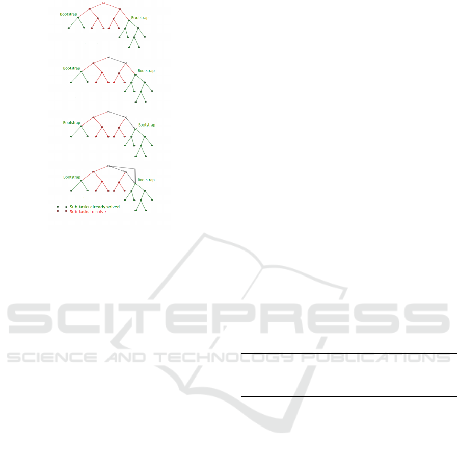
Figure 1: Example of the iterations of DQN-MC-Bootstrap.
are summarized in Algorithm 1 and Figure 1 provides
a visual interpretation.
In a certain way our new algorithm DQN-MC-
Bootstrap is a n-step method with a random n which
corresponds to the random time where we jump from
one element to another of the state space partition.
Note that in doing so, we do not optimize the net-
work for the entire task and then do not need a more
complex architecture for the higher dimension task.
4.5 Baseline Algorithms
Breiman Algorithm. We will call Breiman policy,
the classic greedy algorithm which consists in choos-
ing at each node the features which minimize the aver-
age entropy of the target (Breiman et al., 1984). More
precisely ∀s ∈ S: π
Breiman
(s) = arg max
a∈A
H(D | s)−
E[H(D | s,a)].
The quantity maximized is the information gain,
it measures the average loss of uncertainty about the
target outcome that produces action a.
Our Baseline: An Energy-based Policy with Hand-
-crafted Features. As long as the environment P is
well known and fixed, the optimal policy π
?
is de-
terministic. Nevertheless in our application it can be
interesting to propose several symptoms to check at
the user instead of a single one. Indeed the physi-
cians might be reluctant to use a decision support
tool which do not let them a part of freedom in their
choice. This is why we consider for our baseline
an energy-based formulation, a popular choice as in
(Heess et al., 2013): π
θ
(s,a) ∝ e
θ
T
φ(s,a)
where π
θ
(s,a)
is the probability to take action a in state s, φ(s,a) is
a feature vector: a set of measures linked with the in-
terest of taking action a when we are in state s. To
be more precise φ(s,a) is a three-dimensional vec-
tor which includes the information gain provided by
action a in state s, but also the probability of pres-
ence of the symptom suggested by action a when be-
ing in state s and finally a binary function indicating
whether the suggested symptom is typical of the cur-
rently most plausible disease.
The proposed π
θ
is equivalent to a neural network
without hidden layer designed with hand-crafted fea-
tures. When properly optimized this policy outper-
forms by construction the Breiman policy. A REIN-
FORCE algorithm (Williams, 1992) with a baseline
to reduce the variance is perfectly suitable in our case
and exhibits good results, see section 5.
5 NUMERICAL RESULTS
For all the experiments, we used the same architec-
ture for the neural networks (see Table 1) and the ε
parameter of our stopping criterion is set to 10
−6
.
Table 1: Neural network architecture for task T
i
. |B
i
| the
number of remaining relevant symptoms to check.
Name Type Input Size Output Size
L1 Embedding Layer |B
i
| 3 × |B
i
|
L2 ReLu 3 × |B
i
| 2 × |B
i
|
L3 ReLu 2 × |B
i
| |B
i
|
L4 Linear |B
i
| |B
i
|
Our Baseline has Quasi-optimal Performances on
Small Subproblems. Figure 2 compares on some
of our subtasks the performance of the two policies
proposed in section 4.5: the energy-based policy and
the classic Breiman policy. We added the true optimal
policies when it was possible to compute the latter, i.e.
when the dimension was small enough.
Our energy-based policy appears to clearly outper-
forms a classic Breiman algorithm and all the more
so as the dimension increases: the average number of
questions to ask may be divided by two in some cases.
On small subproblems where we have been able to
compute the optimal policy, our energy-based policy
appears to be very close to the optimal policy.
DQN-TD is Much More Instable than DQN-MC.
We also implemented the classical DQN algorithm
with TD method: DQN-TD. We kept the main fea-
tures of DQN-MC in order to facilitate their compari-
ICAART 2020 - 12th International Conference on Agents and Artificial Intelligence
480
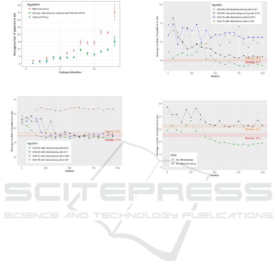
Figure 2: Comparison of Breiman and our energy based-
policy on several subtasks.
Figure 3: DQN-TD vs DQN-MC. Task dimension: 29.
son. The learning rate is initialized with a lower value
than in the DQN-MC algorithm but it is decreased in
exactly the same way in both cases: divided by two
each 300 iterations. Another difference is the frozen
network we use as target in DQN-TD which is not
needed in DQN-MC. We update the frozen network
each 2 iterations (we have also tried to update it less
frequently but have not observed any major differ-
ences with the results presented here).
We compared these two algorithms, DQN-MC
and DQN-TD, on severals of our sub-tasks (see Fig-
ures 3 and 4). We did not observed much difference
on small and intermediate sub-problems: both algo-
rithms converge at the same speed towards solutions
of the same quality. Nevertheless DQN-TD appears
much more sensitive to the learning rate. Indeed as
it can be seen in Figure 3, DQN-TD converge on this
problem, where it remains 29 relevant symptoms to
check and 8 possible diseases, when the learning rate
is initialized at 0.0001. Nevertheless if the learning
rate is chosen a little bit higher, at 0.001, DQN-TD
diverge. On the contrary, DQN-MC converge when
the learning rate is initialized to 0.001 and also when
initialized to 0.01 even if the returns of the algorithm
are less stable in this latter case. These observations
have to be combined with the one of Figure 4 where it
remains 104 relevant symptoms to check and 18 pos-
sible diseases. In this case DQN-TD with an initial
Figure 4: Comparison of DQN-TD, DQN-MC and DQN-
MC-Bootstrap. Task dimension: 104.
Figure 5: Evolution of the performance of the neural net-
work during the training phase. Task dimension: 70.
learning rate of 0.0001 diverge. Reducing the learn-
ing rate to 0.00001 does not change this fact. On the
contrary we do not need to reduce the initial learning
rate of DQN-MC (we take 0.001) to make it converge
to a good solution. Since we have to train as many
neural networks as the number of sub-tasks, we need a
robust algorithm able to deal with different task com-
plexity without changing all the hyper-parameters.
Bootstraping on Already Solved Sub-tasks Helps a
Lot. In these experiments, we compare the perfor-
mance of a simple DQN-MC algorithm against DQN-
MC-Bootstrap on some tasks. The two algorithms use
exactly the same hyper-parameters, the only differ-
ence being the bootstrap trick of DQN-MC-Bootstrap.
Figures 4 and 5 show the benefits of using the
solved sub-tasks as bootstraping methods. In both
cases a simple DQN-MC is unable to find a good solu-
tion while a DQN-MC-Bootstrap outperforms quickly
our baseline. Note that the neural network trained
with DQN-MC-Bootstrap starts with a policy that is
not that bad. It is appreciable as it reduces, since
the beginning of the training phase, the length of the
episodes and then the computing cost associated.
For the experiment of Figure 5 it remains 70 rel-
evant symptoms to check, 9 possible diseases includ-
Optimization of a Sequential Decision Making Problem for a Rare Disease Diagnostic Application
481

ing the disease ”other”, and 20 sub-tasks have been
already solved. For Figure 4 it remains 104 relevant
symptoms to check, 18 possible diseases including
the disease ”other”, and 103 sub-tasks have been al-
ready solved.
Finally we have been able to learn a good policy
for the main task (1) where it remains 220 relevant
symptoms, 82 possible diseases including the disease
”other” and all the possible sub-tasks have been al-
ready solved. Our DQN-MC-Bootstrap starts with a
good policy which needs 45 questions on average to
reach a terminal state and only 40 after some train-
ing iterations. On the contrary, the strategy learned
by DQN-MC trying to solve this task from scratch
must ask on average 117 questions to reach a termi-
nal state and does not improve significantly during the
1000 iterations. The Breiman policy on the global
task needs 89 questions on average to reach a terminal
states (with a variance of 10 questions).
6 CONCLUSION
In this work, we formulated as a stochastic shortest
path problem the sequential decision making task as-
sociated with the objective of building a symptom
checker for the diagnosis of rare diseases.
We have studied several RL algorithms and made
them operational in our very high dimensional envi-
ronment. To do so, we divided the initial task into sev-
eral subtasks and learned a strategy for each one. We
have proven that appropriate use of intersections be-
tween subtasks can significantly accelerate the learn-
ing process. The strategies learned have proven to be
much better than classic greedy strategies.
Finally, a first preliminary study was carried out
internally at Necker Hospital to check the diagnostic
performance of our decision support system. This ex-
periment was conducted on a set of 40 rare disease pa-
tients from a fetopathology dataset, which has no con-
nection to the data used to train our algorithms. We
get good results; indeed more than 80% of the scenar-
ios led to a good diagnosis. Note that theoretically our
definition of the stopping rule of equation (2) makes
impossible any mis-diagnosis as long as ε is chosen
sufficiently low. In practice, of course, mis-diagnosis
are possible because of the inevitable shortcomings of
the environmental model (synonyms, omissions,...).
Research is currently underway to improve and
enrich the environmental model by adding new rare
diseases and symptoms. Finally, we are studying sev-
eral avenues to make our decision support tool more
robust in the face of the unavoidable defects of the en-
vironmental model. A larger scale study is underway
but faces difficulties in obtaining clinical data.
REFERENCES
Amiranashvili, A., Dosovitskiy, A., Koltun, V., and Brox, T.
(2018). Td or not td: Analyzing the role of temporal
differencing in deep reinforcement learning. arXiv.
Besson, R. (2019). Decision making strategy for antenatal
echographic screening of foetal abnormalities using
statistical learning. Theses, Universit
´
e Paris-Saclay.
Besson, R., Pennec, E. L., and Allassonni
`
ere, S. (2019).
Learning from both experts and data. Entropy, 21,
1208.
Breiman, L., Friedman, J. H., Olshen, R. A., and Stone,
C. J. (1984). Classification and Regression Trees.
Wadsworth and Brooks, Monterey, CA.
Chen, Y.-E., Tang, K.-F., Peng, Y.-S., and Chang, E. Y.
(2019). Effective medical test suggestions using deep
reinforcement learning. ArXiv, abs/1905.12916.
Cover, T. M. and Thomas, J. A. (2006). Elements of Infor-
mation Theory (Wiley Series in Telecommunications
and Signal Processing). Wiley-Interscience, New
York, NY, USA.
Hart, P. E., Nilsson, N. J., and Raphael, B. (1968). A for-
mal basis for the heuristic determination of minimum
cost paths. IEEE Transactions on Systems Science and
Cybernetics, 4(2):100–107.
Heess, N., Silver, D., and Teh, Y. W. (2013). Actor-critic
reinforcement learning with energy-based policies. In
Proceedings of the Tenth European Workshop on Re-
inforcement Learning, volume 24, pages 45–58.
K
¨
ohler, S. and al. (2017). The human phenotype ontology
in 2017. In Nucleic Acids Research.
Korf, R. E. (1985). Depth-first iterative-deepening: An op-
timal admissible tree search. Artif. Intell., 27(1):97–
109.
Mnih, V., Kavukcuoglu, K., Silver, D., Graves, A.,
Antonoglou, I., Wierstra, D., and Riedmiller, M. A.
(2013). Playing atari with deep reinforcement learn-
ing. CoRR, abs/1312.5602.
Peng, Y.-S., Tang, K.-F., Lin, H.-T., and Chang, E. (2018).
Refuel: Exploring sparse features in deep reinforce-
ment learning for fast disease diagnosis. In NIPS.
Sutton, R. S. and Barto, A. G. (2018). Introduction to Re-
inforcement Learning. MIT Press, Cambridge, MA,
USA, 2nd edition.
Tang, K.-F., Kao, H.-C., Chou, C.-N., and Chang, E. Y.
(2016). Inquire and diagnose : Neural symptom
checking ensemble using deep reinforcement learn-
ing. In NIPS.
Williams, R. J. (1992). Simple statistical gradient-following
algorithms for connectionist reinforcement learning.
Machine Learning, 8:229–256.
Zubek, V. B. and Dietterich, T. G. (2005). Integrating learn-
ing from examples into the search for diagnostic poli-
cies. CoRR, abs/1109.2127.
ICAART 2020 - 12th International Conference on Agents and Artificial Intelligence
482
