Temporal Cognitive Maps
Adrian Robert, David Genest and Stéphane Loiseau
LERIA, Université d’Angers, France
Keywords:
Cognitive Map, Ontology, Time Representation, Query Language, Semantic Model, OWL.
Abstract:
A cognitive map is an oriented graph whose nodes are labeled by concepts and edges represent influences.
It provides a way to model strategies or influence systems. Cognitive maps do not take into account any
temporal features. This article proposes a solution to this lack: a temporal cognitive map model defined
on a temporal ontology. The temporal ontology is used to represent temporal domain knowledge and to
temporally characterize the concepts of the cognitive map. An extension, named TCMQL, of the cognitive
map query language CMQL, is proposed in order to access the concepts’ temporality and compare them
making inferences.
1 INTRODUCTION
The cognitive map (Axelrod, 1976) model is a se-
mantic model coming from cognitive psychology.
This model is used to represent strategies, or more
generally, influence systems. Cognitive maps are
close to Bayesian networks (Pearl, 2014). While
Bayesian networks focus on the computation of in-
fluences based on conditional probabilities, cogni-
tive maps focus mainly on the visualisation and are
easier to understand for several types of user. A
cognitive map is an oriented graph whose nodes
are labeled by concepts and edges, called influ-
ences, are labeled by an influence value. Influ-
ence values belong to a predefined value set which
can contain symbolic values such as {−,+} (Tol-
man, 1948), {none,some,much,alot} (Kosko, 1986),
or numeric values such as [−1,1] (Kosko, 1986),
{−4,−3,−2,−1, 0,1,2, 3, 4} (Le Dorze, 2013). A se-
quence of influences from a node to another makes
a path. The model can infer a propagated influence
value from a node to another. A taxonomic cogni-
tive map (Le Dorze et al., 2012) is a cognitive map
defined on a taxonomy. The taxonomy organizes the
concepts with ’kind of’ type relations: the nodes of
the taxonomic cognitive map are labeled by concepts
of the taxonomy. The taxonomy can be used to infer
the taxonomic influence value from a concept of the
taxonomy to an other one.
Cognitive maps are used in many fields such as so-
cial sciences (Axelrod, 1976), biology (Martin et al.,
2000) and geography (Çelik et al., 2005). It is typ-
ically the case of the project in geography Kifanlo
1
.
This project aims to study the evolution of the fish-
ing strategies in the Atlantic coast from 1970 to 2016.
About fifty cognitive maps have been designed with
fishermen to model their fishing strategies. Half of
those maps represent fishing strategies in the seven-
ties, the other half represent current fishing strate-
gies, each map contains 25 to 50 nodes. A cognitive
map edition software, VSPCC, has been used and im-
proved
2
.
In the Kifanlo project, there is a significant num-
ber of concepts that have a temporal semantics. These
concepts usually repeat periodically over time like
seasons, fishing seasons and so on... This periodicity
of the concepts should be taken into account in cog-
nitive maps. Notice that the only articles that study
time in cognitive maps stem not on concepts but on
influence : (Park and Kim, 1995; Zhong et al., 2008)
consider the delay or duration process of an influence
in fuzzy cognitive maps.
So, this paper introduces temporal cognitive maps,
which is a new model that extends taxonomic cogni-
tive maps with a temporal ontology for representation
and reasoning.
Because of the periodicity of the concept’s seman-
tics, the temporal ontology aims to represent periodic
intervals (Osmani, 1999). It uses temporal assertions
1
Kifanlo is a project financed by the Fondation de
France. It has been led from 2013 to 2017.
2
The edition software VSPCC (LeDorze and Robert,
2014) has been implemented after the thesis of Aymeric
LeDorze (Le Dorze, 2013), for the project Kifanlo.
58
Robert, A., Genest, D. and Loiseau, S.
Temporal Cognitive Maps.
DOI: 10.5220/0008937300580068
In Proceedings of the 12th International Conference on Agents and Artificial Intelligence (ICAART 2020) - Volume 2, pages 58-68
ISBN: 978-989-758-395-7; ISSN: 2184-433X
Copyright
c
 2022 by SCITEPRESS – Science and Technology Publications, Lda. All rights reserved

that are triples made of two periodic intervals related
by a comparison predicate. The proposed temporal
ontology could be added to other temporal ontologies
of reference like owl-time (Hobbs and Pan, 2006a)
which lacks of such periodic temporal entities.
A temporal cognitive map is defined on a temporal
ontology; it contains a set of temporal assertions that
link the nodes of the cognitive map to the temporal
ontology. The nodes can thus be temporally charac-
terized, meaning that a certain influence holds with
respect to the temporal assertions of its nodes.
To reason with a temporal cognitive map, this ar-
ticle proposes the ’Temporal Cognitive Map Query
Language’ TCMQL, which is an extension of the
query language for cognitive maps CMQL (Robert
et al., 2018). TCMQL is made with two temporal
primitives: TimeInfo and Compare. TimeInfo lets
the user access the periodic interval associated with
a node. Compare infers new information using tem-
poral assertions of nodes and the temporal ontology.
This extension provides a way to use the temporal in-
formation of the model for a further analysis of cog-
nitive maps.
TCMQL, as well as VSPCC extended to temporal
cognitive maps, have been delivered to the researchers
in geography that work in the Kifanlo project for fur-
ther analysis
3
.
This article is composed of three parts. The first
recalls the taxonomic cognitive map model. The sec-
ond introduces the temporal cognitive map model.
The third one presents the TCMQL language.
2 TAXONOMIC COGNITIVE
MAP
A taxonomic cognitive map is a graph whose nodes
and edges are respectively labeled by a concept of a
taxonomy and by an influence value; the taxonomy
aims to organize the concepts. The taxonomy is even
more useful when using a set of cognitive maps, to
make sure that different cognitive maps use the same
concepts (Chauvin et al., 2009).
2.1 Taxonomic Cognitive Map Model
The taxonomy organizes the concepts by specifying
a specialization relation between them.
3
This work is being led in the project Analyse Cognitive
de Savoirs granted by the french region Pays de la Loire
from 2017 to 2020.
Definition 1 (Taxonomy). Let C be a concept set.
A taxonomy T = (C, ≤) is a set of rooted trees of
concepts that represents a partial order relation ≤
whose meaning is ’kind of’.
Example 1. T
1
is the taxonomy of the figure 1. Some
concepts are ordered by a relation of specialization.
For instance, the relation MultiPurposeShip
≤ Ship, meaning that MultiPurposeShip is a
kind of Ship, is represented by an arrow in the figure.
The most specialized concepts of the taxonomy
are said elementary.
Definition 2 (Elementary concepts). Let T = (C,≤)
be a taxonomy. The elementary concepts of T are:
elem
T
= {c ∈ C/ ∀c
0
∈ C,c
0
≤ c =⇒ c
0
= c}.
Example 2. In T
1
(figure 1), the elementary
concepts are elem
T
1
={MultiPurposeShip,
RemoteArea...}; only the concepts Ship,
FishingActivity and Pleasure are not
elementary.
A taxonomic cognitive map is a graph whose
nodes and edges are respectively labeled by an
elementary concept of a taxonomy and an influence
value. The influence value represents the strength
of the influence and belongs to a defined value set
which can be qualitative or quantitative, discrete or
continuous.
Definition 3 (Taxonomic cognitive map). A taxo-
nomic cognitive map defined on a taxonomy T =
(C,≤) and a value set I is an oriented labeled graph
CM=(N,E,labelN,labelE) such that:
• N : the nodes of the graph.
• E ⊂ N × N: the edges are called influences.
• labelN :N → elem
T
is a label function on the
nodes.
• labelE :E → I is a label function on the edges.
Example 3. CC1 and CC2 are the two taxonomic
cognitive maps of the figure 2. They are defined
on the taxonomy T
1
of the figure 1 and the value
set I = [−1,1]. Note that, in the figure, each node
has a unique identifier per map n
1
,n
2
... that is dis-
played only for clarity in this paper. An influence
labeled by 1 (resp. -0.25) means that the source
node influences strongly (resp. weakly) and posi-
tively (resp. negatively) the destination node. In
Temporal Cognitive Maps
59

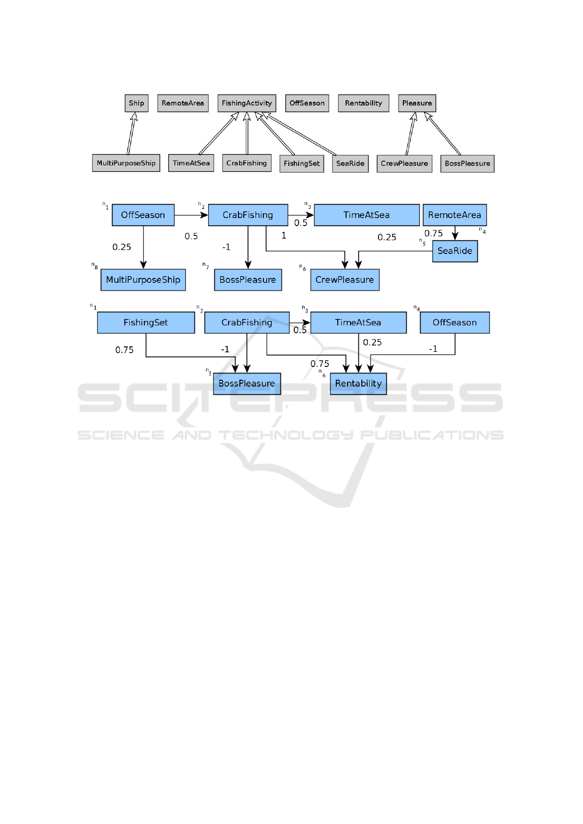
Figure 1: A taxonomy T
1
.
Figure 2: Two taxonomic cognitive maps, CC1 (top) and CC2 (bottom).
our application, each fisherman designs a cogni-
tive map: CC1 has been designed by fisherman1,
and CC2 by fisherman2. In CC2, the node n
2
(CrabFishing) influences strongly and negatively
(-1) the node n
5
(BossPleasure); which means
that the boss does not like fishing crab.
2.2 Taxonomic Cognitive Map Inference
A path is a sequence of influence which represents a
way a node of the map influences another. A path is
said minimal if it does not contain any cycle. Notice
that between two nodes, there can be more than one
minimal path.
Definition 4 (Path). Let CM =(N,E,labelN,labelE) be
a taxonomic cognitive map defined on T = (C,≤)
and I. Let a,b ∈ N be two nodes of CM.
• A path P from a to b is a sequence of length
length
P
≥ 1 of influences (u
i
,u
i+1
) ∈ E (with i ∈
[0;length
P
−1]) such that a = u
0
is the source of P
and b = u
length
P
is the destination of P. This path
is denoted by a → u
1
→ ··· → b.
• A path P is said minimal if ∀i, j ∈ [0; length
P
],i 6=
j ⇒ u
i
6= u
j
.
• The set of all minimal paths on CM is denoted by
Paths
CM
.
Example 4. This example is based on CC2 (figure 2).
p
1
= n
2
(CrabFishing) → n
3
(TimeAtSea) →
n
6
(Rentability) is a minimal path of length=2,
from the source node n
2
to the destination node n
6
.
p
2
= n
2
(CrabFishing) → n
6
(Rentability) is
a minimal path of length=1.
One of the main features of cognitive maps is
their ability to infer the propagated influence from any
node to any other one, which denotes a value of influ-
ence. To do that, every influence path from the node
to the other is involved.
The propagated influence from a node to another
can be calculated differently depending on the map’s
semantics and on the value set on which it is defined.
In all cases, the computation of the propagated influ-
ence first assigns a path value for each path with a
function, then secondly aggregates those values with
an other function.
ICAART 2020 - 12th International Conference on Agents and Artificial Intelligence
60

Definition 5 (Propagated Influence). Let
CM=(N,E,labelN,labelE) be a taxonomic cogni-
tive map defined on T = (C,≤) and I.
• The path value is a function PV
path
: Paths
CM
→ I
which infers the propagated influence of a path.
• The propagated influence value is a function
PV : N × N → I which infers the propagated
influence from a node to another one, aggregating
the path values of each path between the two
nodes.
In this paper, we will use the value set I = [−1,1].
A product function will be used as path value and a
mean function for the propagated influence value as it
is often done in cognitive maps (Genest and Loiseau,
2007).
Example 5. This example is based on CC2 (figure 2).
The paths p
1
and p
2
come from the example 4.
Let’s infer the propagated influence value between
n
2
and n
6
, respectively labeled by CrabFishing
and Rentability. The set of all minimal paths
between those two nodes is Paths
n
2
,n
6
= {p
1
, p
2
}, it
contains two paths. To infer the propagated influ-
ence value between n
2
and n
6
we need PV
Path
(p
1
)
and PV
Path
(p
2
). From the chosen product func-
tion, we have PV
Path
(p
1
) = 0.5 ∗ 0.25 = 0.125 and
PV
Path
(p
2
) = 0.75. Then, aggregating the path
values, PV (n
2
,n
6
) =
(0.125+0.75)
2
= 0.44. So the
propagated influence value from n
2
to n
6
is 0.44.
The taxonomic cognitive map model can also infer
a taxonomic influence value which is used to infer the
influence value between any pair of concepts of the
taxonomy. Note that the propagated influence value
is a particular case of the taxonomic influence value
where the concepts are elementary. The taxonomic
influence value is not presented in this article, but is
described in (Chauvin et al., 2009).
3 TIME REPRESENTATION
This section introduces the periodic intervals, then
proposes a temporal ontology defined on those peri-
odic intervals and temporal assertions that compare
pairs of them. So, the temporal cognitive map can be
introduced, it is a taxonomic cognitive map defined
on a temporal ontology.
3.1 Periodic Intervals
A periodic interval (Ermolayev et al., 2014; Ermo-
layev et al., 2008; Poveda-Villalón et al., 2014; Os-
mani, 1999) is a type of non-convex interval (Lad-
kin, 1986), which is an interval composed of several
unconnected convex subintervals. Periodic intervals
have the particularity to be composed of subintervals
that have the same length and are equally spaced. For
instance ’winter’ is a periodic interval.
The periodic intervals of Osmani and Balbiani (Os-
mani, 1999; Balbiani and Osmani, 2000) that also
considers qualitative relations between them are cho-
sen. This approach is relevant to the Kifanlo project
and, in general, seems suited for cognitive maps as it
offers more flexibility and handles the lack of precise
information.
Definition 6 (Periodic Interval). A periodic interval
is a non-convex interval whose subintervals are
equally spaced and have equal length.
Example 6. January is a periodic interval since
all its subintervals last one month and occur every
year. Summer is also a periodic interval, with subin-
tervals lasting three months and occurring every year.
This paper proposes to specify those periodic
intervals with qualitative relations between two inter-
vals using a comparison predicate. Those predicates
are the 16 relations of Osmani (Osmani, 1999) plus
5 relations. The relations of Osmani are very similar
to the 13 relations of the Allen’s intervals, except
that the precedence and its inverse are replaced by
5 relations which consider the periodicity. This
paper also considers two relations (Inside/Disjoint)
that combine some of Osmani’s relations and three
relations (<,>,=) that compare duration of intervals,
which can not be done with Osmani’s intervals.
Definition 7 (Comparison predicate). A com-
parison predicate is a binary relation whose
domain and range are periodic intervals. P
is the set of the 21 comparison predicates:
{m,mi,s,si,d,di,f,fi,o,oi,eq,ppi,mmi,moi,omi,ooi,
in,dis,<,=,>}
The table below shows the 16 relations of Os-
mani & Balbiani, the column meaning explains
the relations through an ordering of the boundaries
(A1,A2,B1,B2) of the periodic intervals A and B. This
ordering comes from the CYCORD theory (Röhrig,
1994). Two added relations are: ’in’(Inside) which
Temporal Cognitive Maps
61

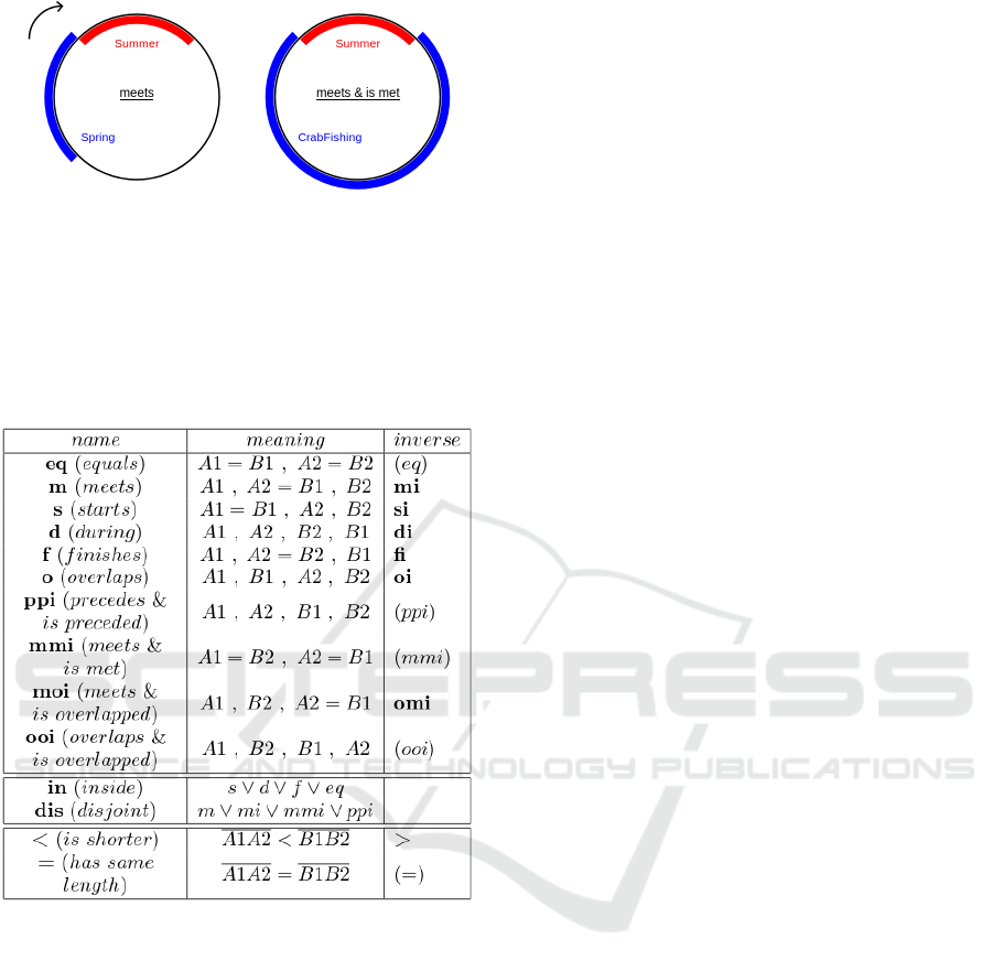
Figure 3: Two cyclic representations of relations between
periodic intervals.
is the disjunction of ’s’,’d’,’f’,’eq’ and ’dis’(Disjoint)
which is the disjunction of ’m’,’mi’,’mmi’,’ppi’.
To these relations are also added three relations to
compare the duration of periodic intervals : ’<’,’>’
and ’=’.
Periodic intervals and comparison predicates
defined above are used to represent temporal knowl-
edge through temporal assertions. A temporal
assertion is an assertion which represents a relation
between two periodic intervals. It is a triple (inter-
val,predicate,interval).
Definition 8 (Temporal assertion). P is the set of
the 21 comparison predicates. A temporal assertion
is an assertion which constitute a triple (e
1
, p, e
2
)
such that p∈ P and e
1
and e
2
are periodic intervals.
Example 7. The relations between periodic intervals
are often represented on a circle (figure 3) which
is to be read clockwise. The first circle represents
the temporal assertion (Spring, meets, Summer) and
it matches the ordering (’SpringBegins’, ’Sprin-
gEnds’=’SummerStarts’, ’SummerEnds’) of the
second line of the table. Its inverse relation is
mi (is met by), so we have (Summer, is met by,
Spring). The second circle illustrates the temporal
assertion (CrabSeason, meets&ismet, Summer).
CrabSeason is related to Summer by the relation
’meets&ismet’ which means that the crab season
starts when summer ends and ends when summer
starts. Some comparison predicates are used to
compare duration, for instance in the temporal
assertion (Day, <, Month) the comparison predicate
’<’ is used to compare the duration of Day and
Month.
3.2 Time Ontology
Many temporal ontologies exist, amongst those
owl-time ontology (Hobbs and Pan, 2006b) is a W3C
reference and one of the most used. It turns out that
time ontologies do not take into account periodic
intervals and certainly not the qualitative relations to
compare them. That is why this paper introduces a
new temporal ontology that considers periodic inter-
vals and could be added to existing heavier temporal
ontologies like owl-time. Our light-weight temporal
ontology is composed of the class PeriodicInterval,
the 21 comparison predicates as object properties,
a set of instances of PeriodicInterval and a set of
temporal assertions on these individuals.
Definition 9 (Temporal Ontology). A temporal ontol-
ogy O = (P, E ,A ) is an ontology such that :
• P is the set of the comparison predicates.
• E is a set of periodic intervals.
• A is a set of temporal assertions of the ontology.
Example 8. The figure 4 represents the temporal on-
tology O
1
. The periodic intervals of this ontology are
E ={Spring, CrabSeason, Year ...} and the temporal
assertions are A = {(Season,<,Year), (CrabSeason,
meets&ismet, Summer)...}.
3.3 Temporal Cognitive Map
A temporal cognitive map is a taxonomic cognitive
map defined on a temporal ontology. Each node of
the map is labeled by a periodic interval and a set
of temporal assertions links those periodic intervals
to the ontology. This way, nodes may be temporally
characterized.
ICAART 2020 - 12th International Conference on Agents and Artificial Intelligence
62

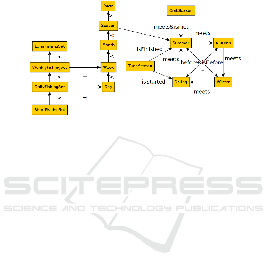
Figure 4: A partial representation of the temporal ontology O
1
.
Definition 10 (Temporal cognitive map). Let
O = (P, E ,A ) be a temporal ontology. Let
CM=(N,E,labelN,labelE) be a taxonomic cogni-
tive map defined on T (C,≤) and I. A temporal
cognitive map TCM defined on O is a triple
(CM,labelT,A
TCM
) such that :
• labelT : is a label function on the nodes of the map
which attaches a unique periodic interval e
n
to a
node n.
• A
TCM
is a set of temporal assertions (e
1
, p, e
2
)
where labelT
−1
(e
1
) ∈ N and e
2
∈ E .
In the next part, a set of temporal cognitive maps
based on the same taxonomy, value set and temporal
ontology is considered. So to specify an associated
periodic interval, the following notation is used.
Notation 1 (Associated Periodic interval). The
periodic interval associated with a node labeled by a
concept ’c’ of a map ’m’ is noted ’m_c’.
Example 9. This example describes the two tempo-
ral cognitive maps of the figure 5: TCM1 and TCM2.
A temporal assertion (in yellow) of a temporal cog-
nitive map is visually represented below the node
(in blue) that it characterizes. The periodic inter-
val attached to the node is visually omitted, that is
why temporal assertions are written as couples and
not triples. For instance in TCM1, the node la-
beled by OffSeason is characterized by the tempo-
ral assertion (TCM1_OffSeason, si, Summer) where
TCM1_OffSeason is the omitted periodic interval at-
tached to this node and ’si’ is the comparison pred-
icate ’isStartedBy’. Notice that several temporal as-
sertions can be attached to the same node, as it is
the case for the node labeled by CrabFishing in
TCM1. This node is characterized by a periodic in-
terval that lasts one month (=,Month) at the end of
the CrabSeason (f,CrabSeason). The fisherman 1
fishes crab for one month at the end of the crab sea-
son.
4 TCMQL
CMQL is a query language whose syntax is close to
the one of SQL and whose semantics is similar to
the one of the relational domain calculus (Louis and
Pirotte, 1982; Robert et al., 2019). CMQL’s particu-
larity resides in the use of many primitives that allow
to access the various features of a taxonomic cognitive
map set. TCMQL is the extension of CMQL that in-
tegrates two temporal primitives, TimeInfo and Com-
pare, which allow to access the concepts’ temporal
assertions and compare them. TCMQL is designed to
query a set of temporal cognitive maps defined on the
same temporal ontology.
4.1 Primitive ’TimeInfo’
The extraction primitive TimeInfo links a cognitive
map, a concept of this map, and the periodic interval
associated with the node labeled by this concept in
this map.
Definition 11 (Primitive: TimeInfo). Let S be a set
of temporal cognitive maps defined on the same tem-
poral ontology O = (P,E , A ), taxonomy T = (C,≤)
Temporal Cognitive Maps
63

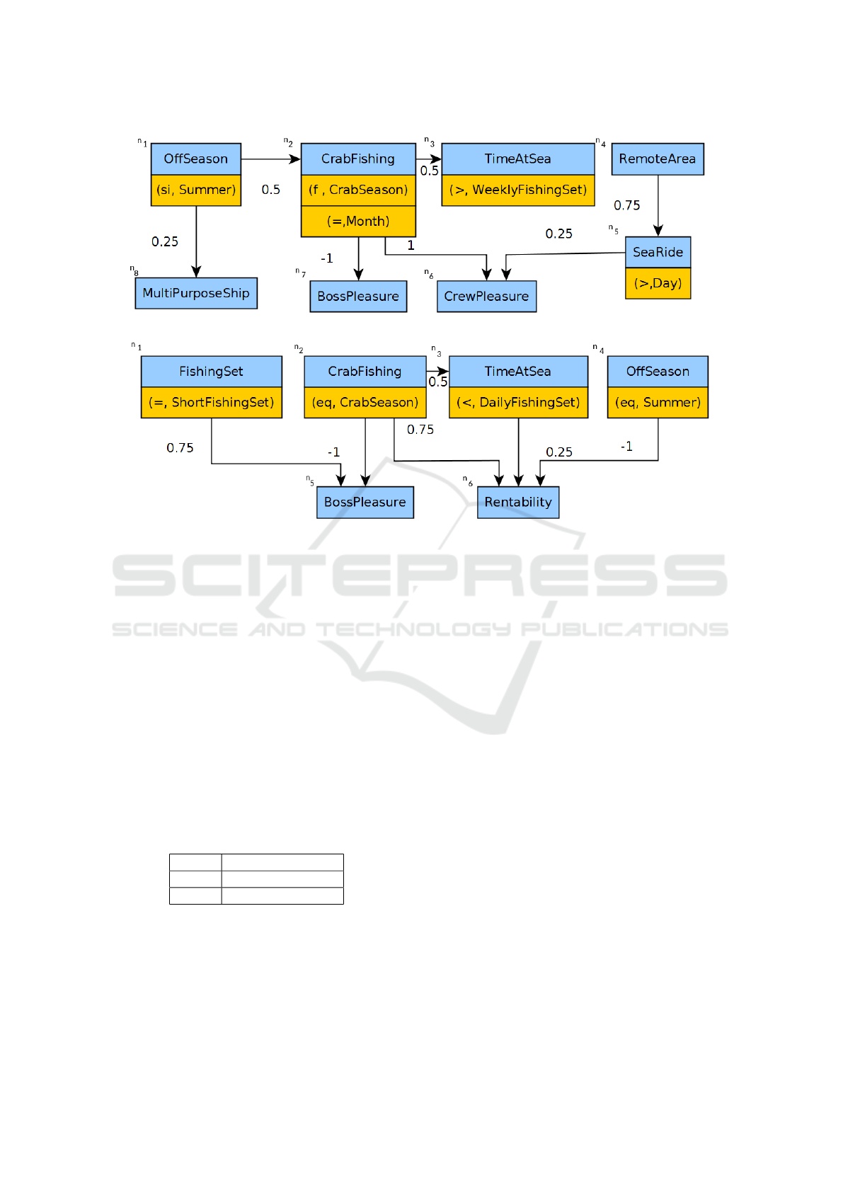
Figure 5: Two temporal cognitive maps, TCM1 (top) and TCM2 (bottom).
and I. Let E
S
be the set of all periodic intervals asso-
ciated with the nodes of the maps in S. The primitive
TimeInfo(map:S, concept:C, interval:E
S
) is a relation
made of the set of the triples (map,concept,interval)
such that ∃n ∈ N
map
,LabelT
map
(n) =interval and
labelN
map
(n) =concept.
Example 10. In TCMQL, a variable is a syntactic ex-
pression prefaced with "?" like in SPARQL (Harris
et al., 2013). The following examples uses the maps
TCM1 and TCM2 (figure 5).
TimeInfo(?map,TimeAtSea,?interval) is a primitive
formula, which is the syntactic expression of a prim-
itive. Its meaning is a binary relation whose value
is the set of tuples (?map,?interval) in which ?inter-
val is associated with the node labeled by the concept
TimeAtSea in ?map :
?map ?interval
TCM1 TCM1_TimeAtSea
TCM2 TCM2_TimeAtSea
The primitive TimeInfo is used here to link
concepts and maps to associated periodic intervals,
TimeAtSea is then used in TCM1 and TCM2.
Used alone the usefulness of this primitive is lim-
ited, it is often used in conjunction with the primitive
Compare defined below.
4.2 Primitive ’Compare’
When the designer of a temporal cognitive map adds
his domain knowledge, he adds the least amount of
temporal assertions and expects the implicit ones to
be taken into account: an inference is thus necessary.
151 inference rules are used for these inferences, they
are OWL2(Hitzler et al., 2009) rules of two types de-
scribed in the next example. The comprehensive list
of rules is not given in the paper as it is too long but
available online (Robert, 2019). The rules about the
16 Balbiani’s relations can be found also in the refer-
ences (Balbiani and Osmani, 2000), a few other rules
about the new predicates are added.
Example 11. Here are some inference rules:
• SubObjectPropertyOf(during inside) which
means (e
1
, during, e
2
)→(e
1
, inside, e
2
)
• SubObjectPropertyOf(starts <) which means (e
1
,
starts, e
2
)→(e
1
, <, e
2
)
• SubObjectPropertyOf(
ObjectPropertyChain(meets startedBy) meets)
which means (e
1
, meets, e
2
) ∧ (e
2
, startedby,
e
3
) → (e
1
, meets, e
3
)
Using the ontology of the figure 4 and the cognitive
maps figure 5, the inference produces assertions like :
ICAART 2020 - 12th International Conference on Agents and Artificial Intelligence
64

• (CrabSeason, disjoint, Summer) which means that
the crab season is outside the summer. This asser-
tion comes from the assertion (CrabSeason, mmi,
Summer) of O
1
and the rule (e
1
, mmi, e
2
)→(e
1
,
disjoint, e
2
).
• (TunaSeason, >, Season) which means that the
season of tuna is longer than a calendar sea-
son. This assertion comes from the assertions (Tu-
naSeason, fi, Summer), (Season, =, Summer) of
O
1
and the rules (e
1
, fi, e
2
)→(e
1
, <, e
2
) and (e
1
,
>, e
2
) ∧ (e
2
,=, e
3
) → (e
1
, >, e
3
).
• (TCM1_CrabFishing, meets, Summer) which
means that Summer starts when the crab season
ends. This assertion comes from the assertions
(TCM1_CrabFishing, f, CrabSeason) of TCM1,
(CrabSeason, mmi, Summer) of O
1
and the rule
(e
1
, f, e
2
) ∧ (e
2
, mmi, e
3
) → (e
1
, meets, e
3
).
Inferences can be carried out on a set that contains
the temporal assertions of the ontology and the
temporal assertions of each temporal cognitive map.
The saturated set is the set of temporal assertions that
can be deduced from all these temporal assertions
and the inference rules.
Definition 12 (Saturated set). Let R a set of rules and
S = {(CM
1
,labelT
1
,A
1
),... ,(CM
k
,labelT
k
,A
k
))}
be a set of k temporal cognitive maps defined on
O = (P,E ,A ), I
S
is the saturated set of temporal
assertions resulting from the inference of the rules of
R on the set A ∪
k
S
i=1
A
i
.
The primitive Compare uses the saturated set
of temporal assertions, it is a relation between two
periodic intervals and a comparison predicate which
is a valid comparison between these intervals.
Definition 13 (Primitive: Compare). Let S be a
set of temporal cognitive maps defined on the same
ontology O = (P, E ,A ) where P is the set of
comparison predicates. Let E
S
be the set all periodic
intervals associated with the nodes of the maps in S.
Let I
S
the saturated set of all temporal assertions.
The primitive Compare(e1: E
S
∪E ,p: P,e2: E
S
∪E )
is a relation made of the triples (e1, p, e2) such that
(e1, p, e2) ∈ I
S
.
Example 12. The following examples use the ontol-
ogy O
1
(figure 4) and the temporal cognitive maps
TCM1 and TCM2 (figure 5).
• Compare(TunaSeason, ?pred,
?interval) is a primitive formula which
aims to compare the periodic interval TunaSea-
son (which is from Spring to Summer according
to O
1
) to any other periodic interval. There are
many result tuples like (>,Summer) since the
summer finishes the TunaSeason:
?pred ?interval
isStarted Spring
isFinished Summer
> Summer
> Week
isFinished TCM2_O f f Season
... ...
• Compare(TCM1_TimeAtSea, ?pred,
Month)
is a primitive formula. There is no
answer since we can not evaluate
the comparison of two durations both
greater than a week (TCM1_TimeAtSea,
>, Week) and (Month, >, Week):
?pred
• Compare(Winter,?pred,CrabSeason)
is a primitive formula. This primitive formula
asks the relations between the Winter and the
CrabSeason. Since the CrabSeason starts at the
end of the summer and ends at its beginning, the
winter is during the CrabSeason and thus shorter.
We obtain the three following tuples:
?pred
during
Inside
<
Although the complexity of the inferences is high
(at least EXPTIME), it has not been a problem in our
system for two reasons. Firstly, a cognitive map is
hand designed and it is a visual model so it is usually
quite a small graph, for instance in the Kifanlo project
a thirty nodes map is a big one. Secondly, the satu-
rated set is precomputed and queries give an answer
in an acceptable time in our application. Neverthe-
less, to go one step further, a study should be done to
evaluate the theoretical complexity and how to face it
depending on maps structure.
4.3 Query Examples
Some primitives of CMQL are recalled here for the
following examples. The primitive IsInMap is one
of them: it is a binary relation whose first attribute
is a map and the second a concept. This primitive is
verified if the concept appears in this map. Path is
an other primitive : it is a relation of four attributes,
Temporal Cognitive Maps
65

a map, two concepts of this map and a path whose
source and destination nodes are labeled by the two
concepts. KindOf is a binary primitive with two
concepts of the taxonomy where the first is a kind
of the second. Value is a relation of four attributes
which links a map, two concepts and the taxonomic
influence value of the first second to the second in
the map. TCMQL’s syntax is close to SQL’s syntax :
SELECT selects variables ?x. . . , FROM indicates the
maps to query and WHERE describes the conditions.
Four examples are given here along with their results
and comments, they are based on T
1
(fig. 1), O
1
(fig. 4) and TCM1,TCM2 (fig. 5).
Example 13. The primitives IsInMap and KindOf
are used in this example. In plain English this query
means : ’In which maps are used the concepts types
of Pleasure?’.
SELECT ?map,?concept FROM TCM1,TCM2
WHERE{
KindOf(?concept, Pleasure)
AND IsInMap(?map,?concept)
}
The first condition allows to obtain the concepts
that are types of Pleasure in the taxonomy. The
second condition gets the couples (map, concept)
such that the concept belongs to the map. The re-
sult of this query is the list of the following tuples
(?map,?concept):
?map ?concept
TCM1 BossPleasure
TCM1 CrewPleasure
TCM2 BossPleasure
The result shows what are the types of the concept
pleasure and in which maps they appear.
Example 14. In plain English this query means
:’When does fisherman1(TCM1) fish crabs in com-
parison to fisherman2(TCM2)?’.
SELECT ?pred FROM TCM1,TCM2 WHERE{
TimeInfo(TCM1, CrabFishing, ?e1)
AND TimeInfo(TCM2, CrabFishing,
?e2) AND Compare(?e1,?pred,?e2)
}
The first two conditions allow to get the temporal
entities of the concept CrabFishing in TCM1 and
TCM2. The third condition allows to get all compar-
ison predicates between those two temporal entities
that are characterized by "finishes CrabSeason" and
" = Month" for the one in TCM1 and by "equals
CrabSeason" for the other. The result is made of the
tuples (?pred):
?pred
f inishes
<
The result shows that the fisherman1 fishes at the
end of the fisherman2’s fishing period, for a shorter
period.
Example 15. In plain English this query means
:’Which duration of FishingSets influences BossPlea-
sure?’.
SELECT ?p, ?e2 FROM TCM1,TCM2
WHERE{
Path(?map,FishingSet,BossPleasure,?path)
AND TimeInfo(?map,FishingSet,?e1)
AND Compare(?e1, ?p, ?e2))}
The first condition allows to get the maps in which
FishingSet influences BossPleasure (TCM2). The two
following conditions allow to get the temporal infor-
mation about FishingSet in the right map.
?p ?e2 ?m
= ShortFishingSet TCM2
< Day TCM2
... ... ...
The result shows that according to the fisherman2
(TCM2), the BossPleasure is influenced by a short
period of fishingset.
Example 16. This query asks the concepts in summer
which influence a concept kind of Pleasure.
SELECT ?map,?c1,?i,?c2
FROM TCM1,TCM2
WHERE{KindOf(?c2,Pleasure) AND
Value(?map,?c1,?c2,?i) AND ?i != 0
AND
TimeInfo(?map,?c1,?e1) AND
Compare(?e1,in,Summer)}
The first condition allows to get all concepts ?c2
kind of Pleasure. The second and third ones allow
to get the concepts ?c1 that influences ?c2 with their
influence value. The two last conditions filter only the
concepts ?c1 in summer.
?map ?c1 ?i ?c2
TCM1 O f f Season −0.5 BossPleasure
TCM1 O f f Season 0.5 CrewPleasure
The results show that, according to the fisher-
man1, the OffSeason which is in Summer influences
negatively the pleasure of the boss and positively the
pleasure of the crew.
ICAART 2020 - 12th International Conference on Agents and Artificial Intelligence
66

5 CONCLUSION
This paper introduces an extension of the cognitive
map model called temporal cognitive map which al-
lows to temporally characterize concepts of the map.
To do this the temporal cognitive map is defined on a
temporal ontology which uses periodic intervals. This
paper proposes also an extension of CMQL, named
TCMQL, which allows to query a set of temporal cog-
nitive map and its new temporal features.
The temporal cognitive map model has been
implemented and tested into the VSPCC soft-
ware which provides tools to edit and use cog-
nitive maps. This software can also execute
TCMQL queries, it is available online (LeDorze
and Robert, 2014). The implementation uses the
temporal ontology owl-time to which is added a
class PeriodicInterval as a subclass of the main
class http://www.w3.org/2006/time#TemporalEntity
and comparison predicates as properties. owl-time
contains other temporal entities, such as instants or
Allen’s intervals. They could also be used once ade-
quate inference rules are added.
The temporal features introduced in this paper
come from real application needs for a better mod-
elling of the fishermen’s strategies and for a more
in-depth analysis in the Kifanlo project. The ACS
project that succeeds the Kifanlo project is currently
in progress, using these new tools.
REFERENCES
Axelrod, R. M. (1976). Structure of decision: the cognitive
maps of political elites. Princeton, NJ, USA.
Balbiani, P. and Osmani, A. (2000). A model for reasoning
about topologic relations between cyclic intervals. In
Principles of Knowledge Representation and Reason-
ing, pages 378–385.
Çelik, F. D., Ozesmi, U., and Akdogan, A. (2005). Par-
ticipatory ecosystem management planning at tuzla
lake (turkey) using fuzzy cognitive mapping. arXiv
preprint q-bio/0510015.
Chauvin, L., Genest, D., and Loiseau, S. (2009). Ontologi-
cal cognitive map. International Journal on Artificial
Intelligence Tools, 18(05):697–716.
Ermolayev, V., Batsakis, S., Keberle, N., Tatarintseva, O.,
and Antoniou, G. (2014). Ontologies of time: Re-
view and trends. International Journal of Computer
Science & Applications, 11(3).
Ermolayev, V., Keberle, N., Matzke, W.-E., and Sohnius, R.
(2008). Fuzzy time intervals for simulating actions.
In International United Information Systems Confer-
ence, pages 429–444. Springer.
Genest, D. and Loiseau, S. (2007). Modélisation, classi-
fication et propagation dans des réseaux d’influence.
Technique et Science Informatiques, 26.
Harris, S., Seaborne, A., and Prud’Hommeaux, E. (2013).
SPARQL 1.1 Query Language. W3C recommenda-
tion.
Hitzler, P., Krötzsch, M., Parsia, B., Patel-Schneider, P. F.,
and Rudolph, S. (2009). Owl 2 web ontology language
primer. W3C recommendation, 27(1):123.
Hobbs, J. R. and Pan, F. (2006a). Time ontology in owl.
W3C working draft, 27:133.
Hobbs, J. R. and Pan, F. (2006b). Time ontology in owl.
W3C working draft, 27:133.
Kosko, B. (1986). Fuzzy cognitive maps. International
Journal of Man-Machines Studies, 24:65–75.
Ladkin, P. B. (1986). Time representation: A taxonomy of
internal relations. In AAAI, pages 360–366.
Le Dorze, A. (2013). Validation, synthèse et paramétrage
des cartes cognitives. PhD thesis, LERIA, Université
d’Angers, France.
Le Dorze, A., Chauvin, L., Garcia, L., Genest, D., and
Loiseau, S. (2012). Views and synthesis of cognitive
maps. In Ramsay, A. and Agre, G., editors, Artifi-
cial Intelligence: Methodology, Systems, and Appli-
cations, pages 119–124, Berlin, Heidelberg. Springer
Berlin Heidelberg.
LeDorze, A. and Robert, A. (2014).
https://sourcesup.renater.fr/projects/vspcc.
Louis, G. and Pirotte, A. (1982). A denotational definition
of the semantics of drc, a domain relational calculus.
In VLDB, pages 348–356.
Martin, B. L., Mintzes, J. J., and Clavijo, I. E. (2000).
Restructuring knowledge in biology: Cognitive pro-
cesses and metacognitive reflections. International
Journal of Science Education, 22(3):303–323.
Osmani, A. (1999). Introduction to reasoning about cyclic
intervals. In Multiple Approaches to Intelligent Sys-
tems, pages 698–706. Springer.
Park, K. S. and Kim, S. H. (1995). Fuzzy cognitive maps
considering time relationships. International Journal
of Human-Computer Studies, 42(2):157–168.
Pearl, J. (2014). Probabilistic reasoning in intelligent sys-
tems: networks of plausible inference. Elsevier.
Poveda-Villalón, M., Suárez-Figueroa, M. C., and Gómez-
Pérez, A. (2014). A pattern for periodic intervals. Se-
mantic Web Journal, pages 1–10.
Robert, A. (2019). http://www.info.univ-
angers.fr/pub/adrian/rules/rules.html.
Robert, A., Genest, D., and Loiseau, S. (2018). A query
language for cognitive maps. In International Confer-
ence on Artificial Intelligence: Methodology, Systems,
and Applications, pages 218–227. Springer.
Robert, A., Genest, D., and Loiseau, S. (2019). The taxo-
nomic cognitive map query language: A general ap-
proach to analyse cognitive maps. In 30th ICTAI,
pages 999–1006. IEEE.
Röhrig, R. (1994). A theory for qualitative spatial reasoning
based on order relations. In Proceedings of the Twelfth
AAAI National Conference on Artificial Intelligence,
AAAI’94, pages 1418–1423. AAAI Press.
Tolman, E. C. (1948). Cognitive maps in rats and men. The
Psychological Review, 55(4):189–208.
Temporal Cognitive Maps
67

Zhong, H., Miao, C., Shen, Z., and Feng, Y. (2008). Tempo-
ral fuzzy cognitive maps. In 2008 IEEE International
Conference on Fuzzy Systems (IEEE World Congress
on Computational Intelligence), pages 1831–1840.
IEEE.
ICAART 2020 - 12th International Conference on Agents and Artificial Intelligence
68