Metrics Performance Analysis of Optical Flow
Taha Alhersh
1 a
, Samir Brahim Belhaouari
2 b
and Heiner Stuckenschmidt
1 c
1
Data and Web Science Group, University of Mannheim, Mannheim, Germany
2
College of Science and Engineering, Hamad Bin Khalifa University, Education City, Doha, Qatar
Keywords:
Performance Analysis, Optical Flow, Metrics.
Abstract:
Significant amount of research has been conducted on optical flow estimation in previous decades. How-
ever, only limited number of research has been conducted on performance analysis of optical flow. These
evaluations have shortcomings and a theoretical justification of using one approach and why is needed. In
practice, design choices are often made based on qualitative unmotivated criteria or by trial and error. In this
paper, novel optical flow performance metrics are proposed and evaluated alongside with current metrics. Our
empirical findings suggest using two new optical flow performance metrics namely: Normalized Euclidean
Error (NEE) and Enhanced Normalized Euclidean Error version one (ENEE1) for optical flow performance
evaluation with ground truth.
1 INTRODUCTION
Optical flow computation is considered a fundamental
problem in computer vision. In fact, it is originated
from the physiological phenomenon of world visual
perception through image formation on the retina, and
this refers to the displacement of intensity patterns
(Fortun et al., 2015). On the other hand, optical flow
can be defined as the projection of velocities of 3D
surface points onto the imaging plane of visual sen-
sor (Beauchemin and Barron, 1995). However, the
relative motion constructed between the observer and
objects of an observed sense only represents motion
of intensities in the image plane, and not necessarily
represents the actual 3D motion in reality (Verri and
Poggio, 1989). A consequent problem emerges that
intensity changes are not necessarily due to objects
displacements in the sense, but can also be caused
by other circumstances such as: changing light, re-
flection, modifications of objects properties affecting
their light emission or reflection (Fortun et al., 2015).
Research paradigms in optical flow estimation have
advanced from considering it as a classical problem
(Horn and Schunck, 1981; Brox and Malik, 2011)
to a higher-level approaches using machine learning
(Wannenwetsch et al., 2017; Sun et al., 2018; Alhersh
and Stuckenschmidt, 2019). For instance, convolu-
a
https://orcid.org/0000-0002-3673-5397
b
https://orcid.org/0000-0003-2336-0490
c
https://orcid.org/0000-0002-0209-3859
tional neural networks (CNNs) is considered to be
state-of-the-art method for Optical flow estimation.
Despite the fact that optical flow estimation meth-
ods have dramatically evolved, the most common
evaluation methodologies are end point error (EPE)
(Otte and Nagel, 1994) and angular error (AE) (Bar-
ron et al., 1994), noting that AE metric is based on
prior work of Fleet and Jepson (Fleet and Jepson,
1990). Even though EPE and AE metrics are popular,
it is unclear which one is better. Moreover, AE penal-
izes errors in regions of zero motion more than mo-
tion in smooth non-zero regions. In addition, there ex-
ists different cases (Figure 1) where EPE gives same
value between various scenarios which will be dis-
cussed later in this paper. The purpose of this paper,
is not to evaluate optical flow estimation methods, but
to create a new evaluation methodology and propose
new metrics for optical flow performance evaluation,
and compare them with existing evaluation metrics.
2 RELATED WORK
Even though many optical flow estimation algorithms
have been proposed, there are few publications on
their performance analysis. Two main approaches
can be used for evaluating optical flow: qualitative
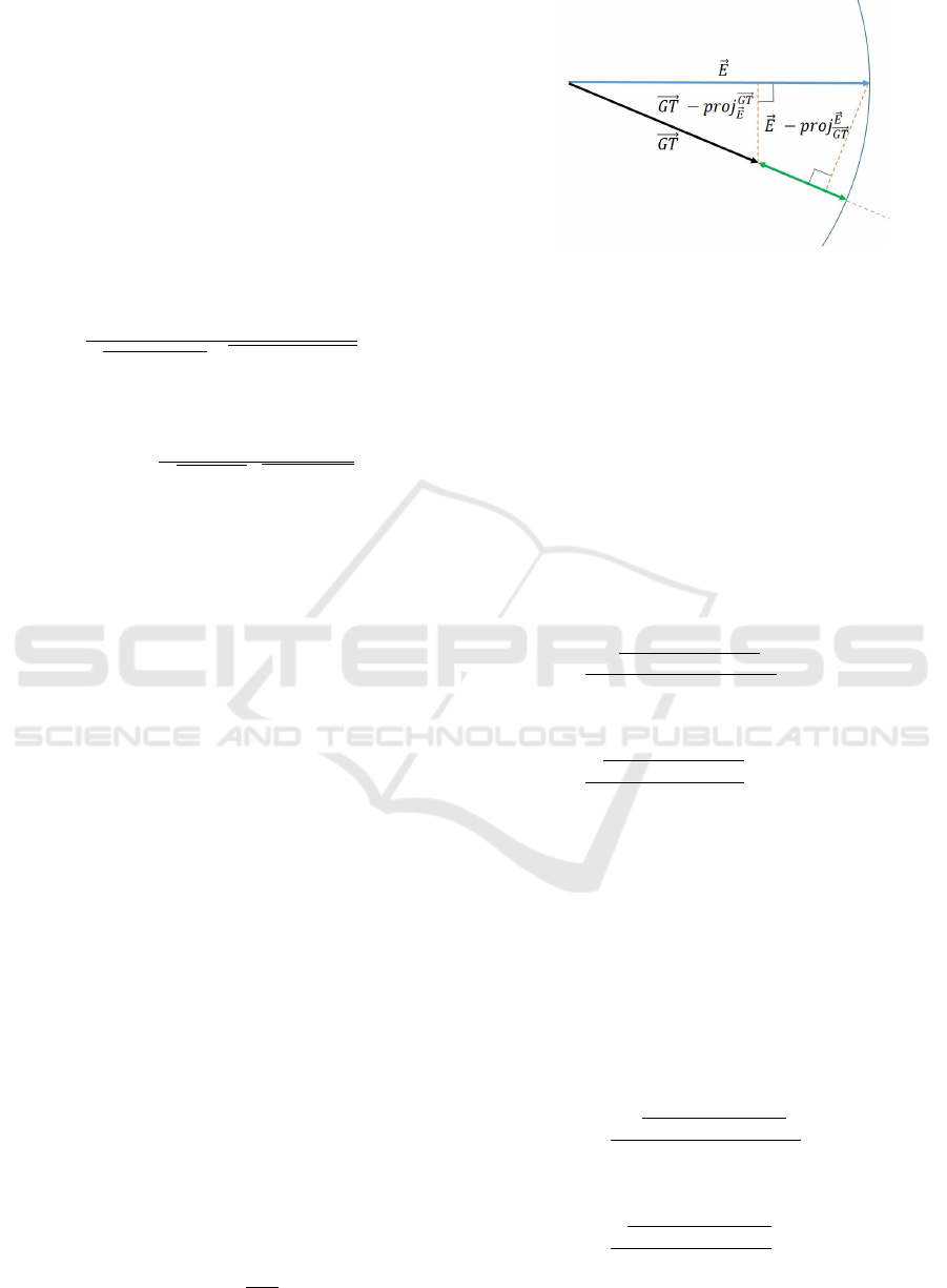
and quantitative. Motion fields of optical flow can be
visualized in either arrow or color forms (Figure 2)
which provide qualitative insights on the accuracy of
Alhersh, T., Belhaouari, S. and Stuckenschmidt, H.
Metrics Performance Analysis of Optical Flow.
DOI: 10.5220/0008936207490758
In Proceedings of the 15th International Joint Conference on Computer Vision, Imaging and Computer Graphics Theory and Applications (VISIGRAPP 2020) - Volume 4: VISAPP, pages
749-758
ISBN: 978-989-758-402-2; ISSN: 2184-4321
Copyright
c
 2022 by SCITEPRESS – Science and Technology Publications, Lda. All rights reserved
749

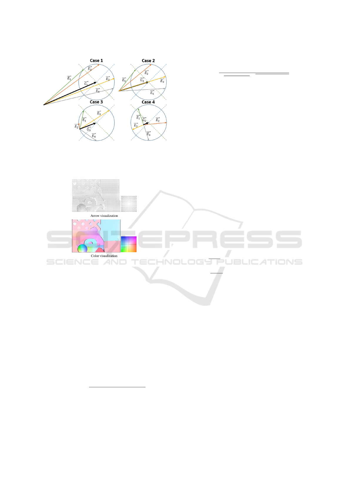
Figure 1: Different cases where the EPE metric gives the
same error value between GT represented by the black vec-
tor
~
G
i
,i ∈(
~
G
1
,
~
G
2
,
~
G
3
,
~
G
4
) and other estimated optical flow
vectors
~
E
j
, j ∈ (
~
E
1
,
~
E
2
,
~
E
3
,
~
E
4
).
Figure 2: Arrow and color visualization of optical flow (For-
tun et al., 2015).
the estimation. Arrow visualization represents mo-
tion vectors and provides good intuition about mo-
tion. On the other hand, motion field vectors should
be under-sampled to prevent arrows overlapping. The
color code visualization allows for dense representa-
tion of motion field via associating color hue to the
direction and saturation to the magnitude of vectors
(Fortun et al., 2015). The first direct quantitative eval-
uation metrics for optical flow were published in 1994
(Otte and Nagel, 1994; Barron et al., 1994) suggest-
ing using EPE (Otte and Nagel, 1994) which can be
described as the Euclidean distance between two vec-
tors; it is defined in Equation 1:
EPE =
q
(u −u
GT
)
2
+ (v −v
GT
)
2
. (1)
and AE (Barron et al., 1994) which represents the
angle between the two extended vectors (1, u, v) and
(1,u
GT
,v
GT
) and defined in Equation 2:
AE = cos
−1

uu
GT
+ vv
GT
+ 1
√
u
2
+ v
2
+ 1
q
u
2
GT
+ v
2
GT
+ 1

. (2)
AE is very sensitive to small estimation errors
caused by small displacements, whereas EPE hardly
discriminates between close motion vectors (Fortun
et al., 2015). Figure 1 illustrates four different cases
when EPE metric gives same error value between
ground truth (GT) and estimated motion vector; this
drawback is caused by the fact that EPE considers
only the difference of vectors and ignores the mag-
nitude of each one.
McCane et al. (McCane et al., 2001) has sug-
gested two evaluation metrics, the first one is defined
in Equation 3, which is based on AE metric with mo-
tion vectors normalization. Nevertheless, AE does not
take into consideration the vector magnitude and uses
only angles, the normalization step has no actual ef-
fect.
E
A
= cos
−1
( ˆc · ˆe), (3)
where E
A
is the error measure, c is GT, e is the esti-
mated optical flow, andˆdenotes vector normalization.
The second metric is the normalized magnitude of
the vector difference between GT and estimated opti-
cal flow which is defined in Equation 4.
E
M
=











kc−ek
kck
if kck >= T ,
|
kek−T
T
| if kck < T and kek >= T ,
0 if kck < T and kek < T ,
(4)
where E
M
is the error measure.
Baker et al. (Baker et al., 2011) compared the per-
formance of EPE and AE and argued that EPE should
become the preferred optical flow evaluation metric
based on a qualitative assessment of an estimated op-
tical flow for Urban sequence.
3 METHOD
In this section, a novel performance evaluation
methodology is proposed, this methodology is based
on using only optical flow ground truths and modified
version for ground truths in terms of shifting horizon-
tally and vertically or magnifying by a certain value,
or rotating or a combination for evaluating perfor-
mance metrics. A description of the used datasets and
mathematical modeling of the proposed metrics are
provided in the consequent sections.
VISAPP 2020 - 15th International Conference on Computer Vision Theory and Applications
750

3.1 Dataset
Three well known datasets have been used for evalu-
ating and analyzing the performance of optical flow.
Since this work is not for evaluating optical flow esti-
mation algorithms, only GT datasets are used.
3.1.1 Baker (Baker et al., 2011)
Baker et al. has proposed new sequences with non-
rigid motion where the ground truth flow is deter-
mined by tracking hidden fluorescent texture. The
number of available GT files is eight and the data de-
scription is shown in Table 1. Three GT files have
maximum values more than 10
9
for limited amount
of pixels which are Dimetrodon, Hydrangea and Rub-
berWhale. To avoid bias in analysis results, a thresh-
old of maximum 10
7
has been set.
3.1.2 KITTI
KITTI dataset is a real-world computer vision bench-
mark. The dataset has two versions, the first one was
proposed in 2012 by (Geiger et al., 2012), and the
second version was proposed by (Menze and Geiger,
2015) in 2015. Compared to KITTI 2012 benchmark,
KITTI 2015 covers dynamic scenes for which ground
truth was established in a semi-automatic process. In
this experiment, only eight random different ground
truths were used.
3.1.3 Sintel
Sintel dataset (Butler et al., 2012) is an open source
synthetic dataset which is extracted from animated
film produced by Ton Roosendaal and the Blender
Foundation. It provides optical flow ground truths as
part of the training set. In this experiment we have
used eight random ground truths for validating pro-
posed and existing optical flow performance metrics.
3.1.4 Modified GT
Different modified versions of GT have been created
based on possible error scenarios. Changes in GT are
based on the the following assumptions.
Lets S = {−30, −20,−10, 10,20, 30}, and for
each GT file, one of the following scenarios is ap-
plied:
1. Shift GT horizontally by s ∈ S and replace shifted
pixels by zeros.
2. Shift GT vertically by s ∈ S and replace shifted
pixels by zeros.
Table 1: Minimum, maximum and standard deviation for
Baker dataset used.
Name Min Max Std
Dimetrodon -4.33E+00 1.67E+09 3.55E+08
Grove2 -3.31E+00 4.01E+00 3.64E+00
Grove3 -4.09E+00 1.43E+01 2.89E+00
Hydrangea -7.02E+00 1.67E+09 4.13E+08
RubberWhale -4.58E+00 1.67E+09 2.09E+08
Urban2 -2.13E+01 8.51E+00 7.96E+00
Urban3 -4.19E+00 1.73E+01 5.15E+00
Venus -9.38E+00 7.00E+00 2.91E+00
3. Shift GT horizontally and vertically by s ∈ S and
replace shifted pixels by zeros.
4. Rotate GT by s ∈ S degrees and replace shifted
pixels by zeros.
5. Magnify GT by multiplying by s ∈ S.
6. Shift GT horizontally and vertically and then ro-
tate by s ∈ S and replace shifted pixels by zeros.
7. Shift GT horizontally and vertically and then ro-
tate and magnify by s ∈ S and replace shifted pix-
els by zeros.
This will allow us to have 42 different versions of
each GT file with total of 336 modified GT files for
each dataset.
3.2 Proposed Performance Metrics
To overcome the drawbacks of the existing optical
flow metrics, we have proposed five different novel
metrics. For each modified optical flow vector
~
E rep-
resented by (u, v) and ground truth vector
~
GT notated
by (u
GT
,v
GT
). The following subsections present the
proposed metrics:
3.2.1 Point Rotational Error (PRE)
AE is adding another dimension and force it to be
equal to 1. From one hand, this will prevent division
by zero, but from the other hand, this will affect the
measurement of the angle. This is an enhancement
on AE, where the angle in 2D space between (u,v)
and (u
GT
,v
GT
) is considered instead of 3D space as
shown in Equation 5:
PRE =

















cos
−1

uu
GT
+vv
GT
√
u
2
+v
2
q
u
2
GT
+v
2
GT

,
if (u
2
+ v
2
) 6= 0 ∧(u
2
GT
+ v
2
GT
) 6= 0
π, if (u
2
+ v
2
) ⊕(u
2
GT
+ v
2
GT
) = 0
0, if (u
2
+ v
2
) = 0 ∧(u
2
GT
+ v
2
GT
) = 0
(5)
Metrics Performance Analysis of Optical Flow
751

for example, if we have the following two points
(0.1,0.1) and (3, 3.1), then AE = 1.2025, but PRE =
0.0164.
3.2.2 Generalized Point Rotational Error
(GPRE)
PRE metric can be generalized when the angle in 3D
space between (α, u,v) and (β,u
GT
,v
GT
) is consid-
ered instead of 3D between (1, u,v) and (1,u
GT
,v
GT
)
space. From Cauchy Schwarz theory (Steele, 2004),
we can prove the following inequalities:
−1 ≤
αβ + (uu
GT
+ vv
GT
)
√
α
2
+ u
2
+ v
2
q
β
2
+ u
2
GT
+ v
2
GT
≤ 1 (6)
The metric GPRE can be defined as:
GPRE =















cos
−1
(
αβ+(uu
GT
+vv
GT
)
√
α
2
+u
2
+v
2
q
β
2
+u
2
GT
+v
2
GT
),
if (u
2
+ v
2
) 6= 0 ∧(u
2
GT
+ v
2
GT
) 6= 0
π, if (u
2
+ v
2
) ⊕(u
2
GT
+ v
2
GT
) = 0
0, if (u
2
+ v
2
) = 0 ∧(u
2
GT
+ v
2
GT
) = 0
(7)
where α and β can be any real numbers, for in-
stance if α = β = 0, then GPRE = PRE. On the other
hand, if α = β = 1 this will led to AE in Equation 2.
3.2.3 Linear Projection Error (LPE)
This metric is a kind of mixture between AE and EPE,
where the magnitude difference between (u, v) and
(u
GT
,v
GT
) is added to the perpendicular distance be-
tween them Figure3. The perpendicular distance be-
tween (u,v) and (u
GT
,v
GT
) is defined as follows:
max

kpro j
~
GT
~
Ek,kpro j
~
E
~
GT k

(8)
where the perpendicular distance is defined as the an-
gular distance between the two non-null vectors
~
E and
~
GT . Therefor our metric can be defined as:
LPE =













k
~
GT −
~
Ek+ max

kpro j
~
GT
~
Ek,kpro j
~
E
~
GT k

,
if k
~
GT ·
~
Ek 6= 0
k
~
GT −
~
Ek+ max

k
~
GT k,k
~
Ek

,
if k
~
GT ·
~
Ek 6= 0
(9)
where the projection of vector
~
b over ~a is given by the
following formula:
pro j
~a
~
b =
~a ·
~
b
|~a|
2
~a (10)
Figure 3: The angular distance between the two non-null
vectors
~
E and
~
GT based on the perpendicular distance be-
tween both vectors.
3.2.4 Normalized Euclidean Error (NEE)
EPE metric is takes into consideration the magnitude
of the difference between two vectors and ignores the
magnitude of each vectors in the sense that the EPE
metric gives the same value for case 1 and case 2
where the radius of two circles is the same (refer to
Figure 1). The following metric is an enhancement of
the magnitude error E
M
proposed by (McCane et al.,
2001):
NEE =



















√
(u−u
GT
)
2
+(v−v
GT
)
2
min

(u
2
+v
2
),(u
GT
2
+v
GT
2
)

,
if min

(u
2
+ v
2
),(u
GT
2
+ v
GT
2
)

> ε
√
(u−u
GT
)
2
+(v−v
GT
)
2
ε
,
if min

(u
2
+ v
2
),(u
GT
2
+ v
GT
2
)

= 0
(11)
where, ε is a threshold around 0.01.
3.2.5 Enhanced Normalized Euclidean Error
(ENEE)
Another way to get over EPE drawbacks is to calcu-
late the relative distance between
~
E and
~
GT vectors
and to use different normalization methods as the fol-
lowing:
ENEE1 =



















√
(k
~
P
GT
k)
2
+τ(k
~
N
GT
k)
2
min

(u
2
+v
2
),(u
GT
2
+v
GT
2
)

,
if min

(u
2
+ v
2
),(u
GT
2
+ v
GT
2
)

> ε
√
(k
~
P
GT
k)
2
+τ(k
~
N
GT
k)
2
ε
,
if min

(u
2
+ v
2
),(u
GT
2
+ v
GT
2
)

= 0
(12)
VISAPP 2020 - 15th International Conference on Computer Vision Theory and Applications
752

If the normalization is performed by only
~
GT vector,
then:
ENEE2 =

















√
(k
~
P
GT
k)
2
+τ(k
~
N
GT
k)
2
q
u
2
GT
+v
2
GT
,
if (u
2
GT
+ v
2
GT
) 6= 0
√
u
2
+ v
2
,
if (u
2
GT
+ v
2
GT
) = 0
(13)
If the normalization is performed by the average of
~
GT and
~
E vectors, then:
ENEE3 =

















2
√
(k
~
P
GT
k)
2
+τ(k
~
N
GT
k)
2
q
u
2
GT
+v
2
GT
+
√
u
2
+v
2
,
if (u
2
GT
+ v
2
GT
) 6= 0
√
u
2
+ v
2
,
if (u
2
GT
+ v
2
GT
) = 0
(14)
If normalization is ignored, then:
ENEE4 =
q
(k
~
P
GT
k)
2
+ τ(k
~
N
GT
k)
2
(15)
where τ is strictly positive value and it works as steer-
ing power for normal component
~
N
GT
and
~
P
GT
and
~
N
GT
are defined as:
~
P
GT
=
(uu
GT
+ vv
GT
)
(u
2
GT
+ v
2
GT
)
~
GT −
~
GT (16)
~
N
GT
=
~
E −
(uu
GT
+ vv
GT
)
(u
2
GT
+ v
2
GT
)
~
GT (17)
4 EXPERIMENTS AND RESULTS
Systematic experiments have been conducted to eval-
uate optical flow performance. As we are evaluating
10 different metrics, a total number of 3360 experi-
ments have been performed for each dataset. Behav-
ior and sensitivity of every metric have been reported
for motion variations in horizontal, vertical, rotational
and magnification or a combination. Parameter set-
tings used in all experiments are summarized in Ta-
ble 2.
As a rule of thumb, a good metric has to produce
an error value proportional to the absolute values in
step sequence S described in Section 3.1.4. A gen-
eral overview of mean error curves for existing and
proposed error metrics in log scale are illustrated in
Figure 4. It is obvious that some metrics are outper-
forming others but yet it’s not clear which metrics are
more suitable for optical flow performance measure.
More detailed explanations and results are re-
ported in the following sections.
Table 2: Metric settings used in all experiments.
Metric Setting
GPRE α = β = 0
NEE ε = 0.01
ENEE1 ε = 0.01,τ = 3
ENEE2 τ = 100
ENEE3 τ = 100
ENEE4 τ = 5
4.1 Metrics Evaluation on Baker
Dataset
Metrics are calculating errors between GT and mod-
ified GT. The most general example for a modified
GT is when GT values are shifted horizontally and
vertically then rotated after magnification by a value.
For instance, Figure 5 is showing mean error metric
curves for Baker dataset. X −axis is representing
values used to shift, rotated and magnify actual GT,
while Y −axis is the mean error values.
Based on our rule of thumb, Figure 5 is showing
that LPE, ENEE4 and EPE metrics are more sensitive
to motion variation when GT is modified with nega-
tive values, while NEE and ENEE1 is more sensitive
to motion variation when GT is modified with positive
values.
According to the approach used in modifying GT,
no motion pixels are replaced with zero values when
GT is rotated, hence, this will increase zero values
in modified GT and mean error would be biased. To
overcome this issue, The third quartile of the error
can be used instead of mean error. The third quartile
is denoted by Q3 , which is the median of the upper
half of the data set. This means that about 75% of the
numbers in the data set lie below Q3 and about 25%
lie above Q3.
Since it is not clear from mean error which metric
is better, Q3 mean error gives a more clear idea about
the best metrics. Figure 6 illustrates Q3 mean error for
all metrics. It is obvious that NEE and ENEE1 metrics
are outperforming other metrics. In the second place,
ENEE4, EPE and LPE metrics. On the third place
ENEE2 and Em metrics.
Visualization of optical flow error for Hydrangea
sample which is part of Baker dataset is shown in Fig-
ure 9 and indicates that NEE and ENEE1 metrics are
compromised metrics between EPE which highly pe-
nalize errors and AE which less penalize errors.
Metrics Performance Analysis of Optical Flow
753

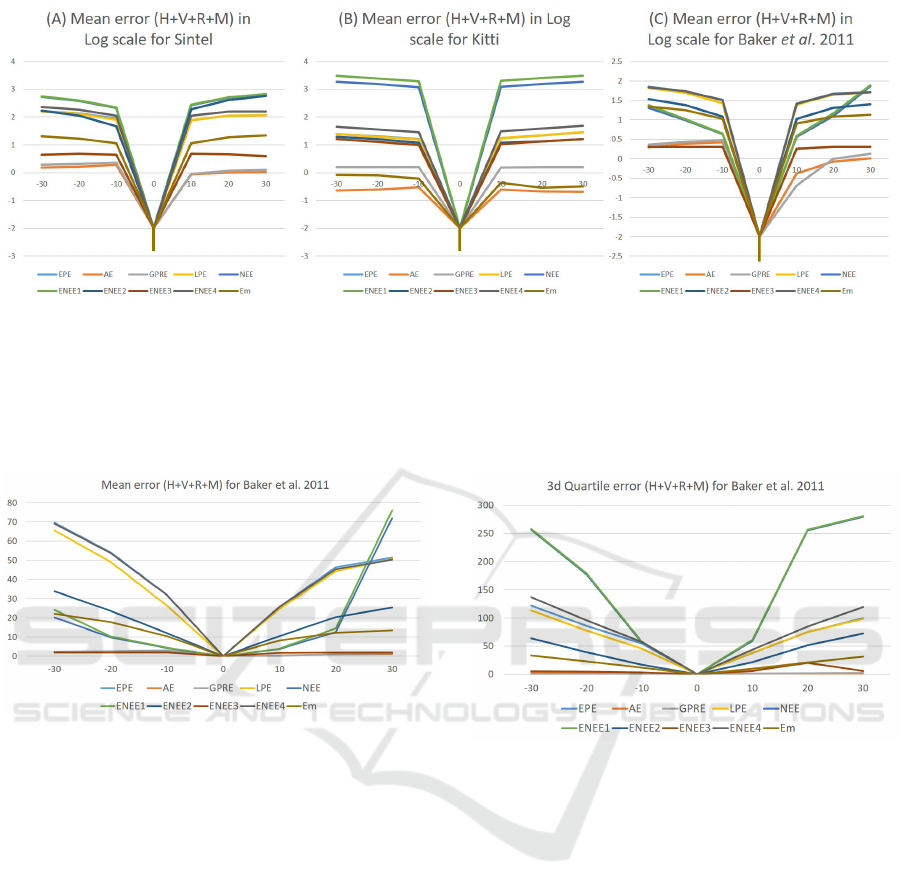
Figure 4: Mean error (y −axis) in log scale for all metrics between GT and modified GT in different scenarios: (I) when GT
are shifted horizontally(H) by number of pixels in x −axis, (II) GT are shifted vertically (V) by number of pixels in x −axis,
(III) GT are magnified (M) by values in x−axis, (IV) GT are shifted horizontally and vertically by number of pixels in x −axis,
(V) GT are rotated (R) by angle degree in x −axis, (VI) GT are shifted horizontally and vertically then rotated by values of
x −axis. For (A) Sintel dataset, (B) Kitti dataset and (C) Baker dataset. Note that log(0
+
) = −∞ which is represented by the
lowest point in the graph.
Figure 5: Mean error (y−axis) for Baker dataset for all met-
ric calculations between GT and modified GT when they
are shifted horizontally and vertically then rotated after that
magnified by values of x −axis.
4.2 Metrics Evaluation on KITTI
Dataset
The second evaluation was conducted on KITTI
dataset. The mean error of existing and proposed met-
rics are shown in Figure 7. It’s clear that ENEE1 and
NEE metrics are more sensitive to motion variation
than other metrics.
Optical flow error visualization for sample image
of KITTI dataset is shown in Figure 10. A compro-
mised visualization between between EPE and AE
metrics are represented by NEE and ENEE1 metrics.
4.3 Metric Evaluation on Sintel Dataset
The last evaluation for metrics was performed on Sin-
tel dataset. The mean error of all metrics is plot-
ted in Figure 8. Based on our rule of thumb, NEE
Figure 6: Third quartile of mean error (y −axis) for Baker
dataset for all metrics calculating error between GT and
modified GT when motion is shifted horizontally and verti-
cally then rotated after that magnified by values of x −axis.
and ENEE1 metrics are producing error values more
proportional to the absolute value of motion change.
Hence, NEE and ENEE1 metrics are more sensitive
to errors and performing better than other metrics.
Visualization of optical flow error as sample im-
age of Sintel dataset is shown in Figure 11. This in-
dicates that NEE and ENEE1 metrics are moderate
versions between between EPE which highly penal-
ize errors and AE which less penalize errors.
4.4 Discussion
A qualitative assessment (Baker et al., 2011) has been
conducted on two common error metrics EPE and
AE, and suggested using EPE rather than using AE
based on only one sample from Baker dataset from
Urban sequence. However, there is a need for a sys-
VISAPP 2020 - 15th International Conference on Computer Vision Theory and Applications
754

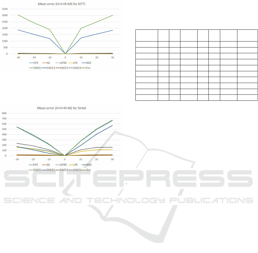
Figure 7: Mean error (y −axis) for KITTI dataset for all
metric calculations between GT and modified GT when
they are shifted horizontally and vertically then rotated after
that magnified by values of x −axis.
Figure 8: Mean error (y−axis) for Sintel dataset for all met-
ric calculations between GT and modified GT when they
are shifted horizontally and vertically then rotated after that
magnified by values of x −axis.
tematic evaluation of optical flow performance, hence
this experiment has been conducted on three popular
datasets using ten different error metrics. A good met-
ric is considered to be more sensitive to errors. For
example, producing error values proportional to the
change of motion between modified GT and GT.
Existing metrics such as EPE, AE and EM have
sensitivity differ slightly from one dataset to another.
For instance, EPE and EM performed good on Baker.
While AE and Em are less sensitive on Kitti and AE
is not sensitive on Sintel. EPE best sensitivity was on
Kitti, on the other hand, AE sensitivity was the worse
among all three metrics.
A detailed look into metrics behavior related to
motion change is illustrated in Figure 12. The follow-
ing observations have been derived:
• It is observed from Figure 12 (A,B and C) that
almost all metrics except ENEE2 and Em are sen-
sitive to horizontal, vertical and (horizontal and
vertical) motion variation, with some differences
in magnitude. ENEE2 and Em metrics are more
sensitive for horizontal variation Figure 12(B) and
Table 3: A summarized results for our rule of thumb method
to choose best metric based on metric sensitivity to mo-
tion variation in horizontal (H), vertical(V), rotational(R)
and magnification (M) or a combination.
V H H+V R M H+V H+V
+R +R+M
EPE X X X X
AE X X X X
GPRE X X X X
LPE X X X X
NEE X X X X X X X
ENEE1 X X X X X X X
ENEE2 X X X X
ENEE3 X X X X
ENEE4 X X X X
Em X X X X
horizontal and vertical variation Figure 12(C).
• All metrics except AE, GPRE and ENEE3 are
sensitive to magnitude of motion variation. AE,
GPRE and ENEE3 metrics can not detect vari-
ations in motion magnitude as shown in Fig-
ure 12(E).
• NEE and ENEE1 metrics are sensitive for angle
variation as seen in Figure 12 (D,F), while AE,
GPRE, and Em are sensitive only for small rota-
tional variation.
Based on the previous observations, we conclude
that all metrics are sensitive to horizontal, vertical and
(horizontal and vertical) variation. AE, GPRE, NEE
and ENEE1 metrics are sensitive to rotational varia-
tions. All metrics except AE and GPRE are sensitive
to magnitude changing in motion. And only NEE and
ENEE1 metrics are sensitive for all horizontal, ver-
tical, rotational, magnitude or a combination. These
results are summarized in Table 3.
5 CONCLUSION
In this paper, a novel performance measure of opti-
cal flow have been proposed. Moreover, a system-
atic evaluation of optical flow performance have been
conducted. Drawbacks of existing performance met-
rics have been identified. Among the five proposed
optical flow performance metrics, NEE and ENEE1
error metrics have outperformed all other metrics in-
cluding the existing ones. The sensitivity of NEE and
ENEE1 to motion variation is very high, indicating
that NEE and ENEE1 error metrics are strongly rec-
ommended to be used for measuring the performance
of estimated optical flow with regard to ground truth.
Metrics Performance Analysis of Optical Flow
755

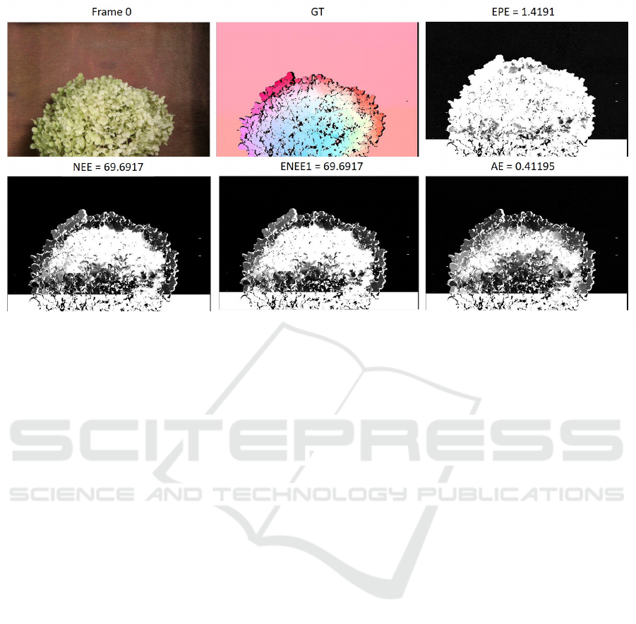
Figure 9: Sample image from Bakers’ (Hydrangea) dataset, the corresponding ground truth and the visualization of motion
error for four different error metrics (EPE, AE, NEE and ENEE1) between ground truth and modified ground truth when GT
pixels are shifted vertically by -50 pixels.
REFERENCES
Alhersh, T. and Stuckenschmidt, H. (2019). Unsupervised
fine-tuning of optical flow for better motion boundary
estimation.
Baker, S., Scharstein, D., Lewis, J., Roth, S., Black, M. J.,
and Szeliski, R. (2011). A database and evaluation
methodology for optical flow. International Journal
of Computer Vision, 92(1):1–31.
Barron, J. L., Fleet, D. J., and Beauchemin, S. S. (1994).
Performance of optical flow techniques. International
journal of computer vision, 12(1):43–77.
Beauchemin, S. S. and Barron, J. L. (1995). The computa-
tion of optical flow. ACM computing surveys (CSUR),
27(3):433–466.
Brox, T. and Malik, J. (2011). Large displacement optical
flow: descriptor matching in variational motion esti-
mation. IEEE transactions on pattern analysis and
machine intelligence, 33(3):500–513.
Butler, D. J., Wulff, J., Stanley, G. B., and Black, M. J.
(2012). A naturalistic open source movie for opti-
cal flow evaluation. In A. Fitzgibbon et al. (Eds.),
editor, ECCV, Part IV, LNCS 7577, pages 611–625.
Springer-Verlag.
Fleet, D. J. and Jepson, A. D. (1990). Computation of com-
ponent image velocity from local phase information.
International journal of computer vision, 5(1):77–
104.
Fortun, D., Bouthemy, P., and Kervrann, C. (2015). Optical
flow modeling and computation: a survey. Computer
Vision and Image Understanding, 134:1–21.
Geiger, A., Lenz, P., and Urtasun, R. (2012). Are we ready
for autonomous driving? the kitti vision benchmark
suite. In CVPR.
Horn, B. K. and Schunck, B. G. (1981). Determining optical
flow. Artificial intelligence, 17(1-3):185–203.
McCane, B., Novins, K., Crannitch, D., and Galvin, B.
(2001). On benchmarking optical flow. Computer Vi-
sion and Image Understanding, 84(1):126–143.
Menze, M. and Geiger, A. (2015). Object scene flow for
autonomous vehicles. In CVPR.
Otte, M. and Nagel, H.-H. (1994). Optical flow estimation:
advances and comparisons. In European conference
on computer vision, pages 49–60. Springer.
Steele, J. M. (2004). The Cauchy-Schwarz master class: an
introduction to the art of mathematical inequalities.
Cambridge University Press.
Sun, D., Yang, X., Liu, M.-Y., and Kautz, J. (2018). Pwc-
net: Cnns for optical flow using pyramid, warping,
and cost volume. In Proceedings of the IEEE Con-
ference on Computer Vision and Pattern Recognition,
pages 8934–8943.
Verri, A. and Poggio, T. (1989). Motion field and optical
flow: Qualitative properties. IEEE Transactions on
pattern analysis and machine intelligence, 11(5):490–
498.
Wannenwetsch, A. S., Keuper, M., and Roth, S. (2017).
Probflow: Joint optical flow and uncertainty estima-
tion. In Computer Vision (ICCV), 2017 IEEE Interna-
tional Conference on, pages 1182–1191. IEEE.
VISAPP 2020 - 15th International Conference on Computer Vision Theory and Applications
756

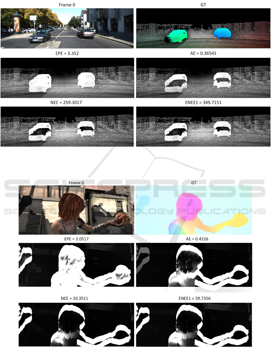
Figure 10: Sample image from KITTIs’ dataset, the corresponding ground truth and the visualization of motion error for four
different error metrics (EPE, AE, NEE and ENEE1) between ground truth and modified ground truth when GT pixels are
shifted vertically by -50 pixels.
Figure 11: Sample image from Sintels’ dataset, the corresponding ground truth and the visualization of motion error for four
different error metrics (EPE, AE, NEE and ENEE1) between ground truth and modified ground truth when GT pixels are
shifted vertically by -50 pixels.
Metrics Performance Analysis of Optical Flow
757

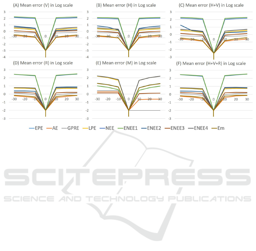
Figure 12: All datasets mean error (y −axis) in log scale for all metrics between GT and modified GT in different scenarios:
(A) when GT are shifted horizontally(H) by number of pixels in x−axis, (B) GT are shifted vertically (V) by number of pixels
in x−axis, (C) GT are magnified (M) by values in x −axis, (D) GT are shifted horizontally and vertically by number of pixels
in x −axis, (E) GT are rotated (R) by angle degree in x −axis, (F) GT are shifted horizontally and vertically then rotated by
values of x −axis. Note that log(0
+
) = −∞ which is represented by the lowest point in the graph.
VISAPP 2020 - 15th International Conference on Computer Vision Theory and Applications
758