Loads Estimation using Deep Learning Techniques in Consumer
Washing Machines
Alexander Babichev
2
, Vittorio Casagrande
4
, Luca Della Schiava
2
, Gianfranco Fenu
1
, Imola Fodor
2
,
Enrico Marson
2
, Felice Andrea Pellegrino
1
, Gilberto Pin
2
, Erica Salvato
1
, Michele Toppano
2
and Davide Zorzenon
3
1
Department of Engineering and Architecture, University of Trieste, Italy
2
Electrolux Italia S.p.A., Porcia, 33080, Italy
3
Technische Universit
¨
at Berlin, Control Systems Group, Einsteinufer 17, D-10587 Berlin, Germany
4
Department of Electrical and Electronic Engineering, University College London, U.K.
Keywords:
Long Short Term Memories, One-dimensional Convolutional Neural Networks, Virtual Sensing.
Abstract:
Home appliances are nowadays present in every house. In order to ensure a suitable level of maintenance,
manufacturers strive to design a method to estimate the wear of the single electrical parts composing an
appliance without providing it with a large number of expensive sensors. With this in mind, our goal consists
in inferring the status of the electrical actuators of a washing machine, given the measures of electrical signals
at the plug, which carry an aggregate information. The approach is end-to-end, i.e. it does not require any
feature extraction and thus it can be easily generalized to other appliances. Two different techniques have been
investigated: Convolutional Neural Networks and Long Short-Term Memories. These tools are trained and
tested on data collected on four different washing machines.
1 INTRODUCTION
Nowadays each house is provided with many differ-
ent appliances of common use. The quality of such
machines is based not only on their efficacy and ef-
ficiency, but also on their reliability. Hence the ca-
pability to ensure an adequate level of maintenance
is something that companies strive for. In particular,
predictive maintenance aims to schedule the replace-
ment of components before their actual break down.
One way to monitor an appliance is providing it with
many sensors that report wear. Even though this
method can be effective, it has the drawback of being
expensive. Hence, another monitoring method should
be found. Electrical signals drawn from the grid are
rather easy physical quantities to measure in electri-
cal appliances, for instance employing a metering de-
vice with computational capabilities able to host e-AI
applications. Finding a reliable method to use such
information to infer the usage of an appliance is of
particular interest. In the present paper, a method
based on deep learning is proposed to estimate the
status of some loads inside a consumer washing ma-
chine. Here, by “load” we mean any appliance’s in-
ternal component (for instance, the heater) that em-
ploys electrical energy. To the best of our knowledge,
such techniques have never been used for this specific
application. However, deep learning techniques have
been employed for similar tasks.
In (Susto et al., 2018) machine learning tools are
used to estimate the weight of clothes inside a wash-
ing machine. The estimated weight is then used by
the washing machine to improve the washing pro-
cess. The approach is based on tools such as ran-
dom forest and logistic regression, which require
handcrafted features. Estimation and machine learn-
ing techniques have been extensively used for Non-
Intrusive Load Monitoring (NILM), that is, estima-
tion of usage of home appliances taking as input elec-
trical signals of the main panel. Different solutions
have been proposed in literature, usage of decision
trees (Maitre et al., 2015), harmonic analysis (Djord-
jevic and Simic, 2018), empirical mode decompo-
sition (EMD) principle (Huang et al., 2019) and k-
Nearest Neighbor classifiers (Alasalmi et al., 2012).
All of these methods require a feature design process
Babichev, A., Casagrande, V., Della Schiava, L., Fenu, G., Fodor, I., Marson, E., Pellegrino, F., Pin, G., Salvato, E., Toppano, M. and Zorzenon, D.
Loads Estimation using Deep Learning Techniques in Consumer Washing Machines.
DOI: 10.5220/0008935104250432
In Proceedings of the 9th International Conference on Pattern Recognition Applications and Methods (ICPRAM 2020), pages 425-432
ISBN: 978-989-758-397-1; ISSN: 2184-4313
Copyright
c
 2022 by SCITEPRESS – Science and Technology Publications, Lda. All rights reserved
425

based on prior knowledge of the functioning of the ap-
pliance. An effective method to overcome this prob-
lem is proposed in (Mocanu et al., 2016) and in (Kim
et al., 2017), where the employment of deep learning
tools is proposed which do not require any feature de-
sign. The aim is to detect the energy consumption of
each appliance of an household, from aggregate mea-
surements of voltage and/or current in the distribution
system.
In the present paper, we employ measurements
of electrical signals of a single appliance, and we
face the problem of load estimation, that encompasses
both regression and classification, in a supervised
learning fashion. In particular, a dataset of signals
acquired during 502 washing cycles, corresponding
to a total of 1002.4 hours of operation has been col-
lected, along with the actual loads status. To deal with
the estimation problem, the deep learning tools which
have been employed are Long Short-Term Memories
(LSTM) and Convolutional Neural Networks (CNNs)
(Goodfellow et al., 2016). LSTM deal natively with
sequential data. As for the CNNs, we employ one
dimensional CNNs, that recently have been proven
effective in time series classification (Hannun et al.,
2019). The remainder of the paper is organized as
follows. Section 2 describes the dataset and the
data preparation. Section 3 specifies the regression
and classification problems and establishes the per-
formance indices. The adopted solution is described
in detail in Section 4 and the experimental results are
reported in Section 5. Conclusions are drawn in Sec-
tion 6.
2 DATASET DESCRIPTION
The required dataset for training and testing the net-
work has to contain enough information to allow the
network generalization capability. Hence, to collect
data, a measurement campaign has been performed on
different washing machines and washing cycles. A to-
tal number of 502 sequences have been collected from
real appliances trying to cover the largest number of
operation settings, 402 of which to be used for train-
ing and the remaining 100 for testing. In order to en-
sure that training and testing sets contained a uniform
level of information, the dataset splitting has been
done once by manually labelling the sequences as
training or testing sequence. Each recorded sequence
contains measured values of the following electrical
quantities:
• real and imaginary parts of I, III, V current har-
monics;
• real and imaginary parts of I, III, V voltage har-
monics;
• cumulative energy drawn from the grid;
and of the following loads:
• drum speed (absolute value in rpm);
• heater (boolean);
• drain pump (boolean);
• electrovalves (boolean).
The aim of this work is to provide a punctual es-
timation of the drum speed and of the boolean (ac-
tivation) status of the last three output variables (0 =
OFF, 1 = ON). Considering that the loads are powered
by electricity, we expect a causal effect (which can be
non-linear and not easy to estimate without adequate
knowledge of the appliance) of the variations of the
state of the loads on the variations of the electrical
quantities. Hence a binary classifier has been trained
for each one of the three boolean loads, whereas the
estimation of the drum speed has been treated as a re-
gression problem. The main issue encountered with
this dataset is that the loads are turned OFF during
most of the time of each recorded cycle. In table 1 the
percentage of ON and OFF samples for each load of
the dataset is shown.
Table 1: Percentage of ON and OFF samples for each load.
OFF samples ON samples
Heater 86% 14%
Drain Pump 87% 13%
Electrovalves 98% 2%
Class unbalance has a detrimental effect in train-
ing (Buda et al., 2018; Grangier et al., 2009). In sec-
tion 4 the employed methods to deal with class unbal-
anced are presented.
2.1 Data Preparation
Recorded sequences include heterogeneous physical
quantities which may have different orders of mag-
nitude. Hence measurements have been normalized
using z-score standardization, i.e., each input sample
of channel i (x
i
), is normalized using the following
formula:
X
i
=
x
i
− µ
i
σ
i
where µ
i
and σ
i
are the sample mean and standard
deviation of the training sequences of the considered
physical quantity (e.g. real part of the first current
harmonic, etc.) and are referred to as normalization
factors.
ICPRAM 2020 - 9th International Conference on Pattern Recognition Applications and Methods
426

In order to make use of CNNs for load classifi-
cation, the dataset requires to be elaborated with an
operation which will be referred to as segmentation
in this paper. This is due to the fact that Convolu-
tional Neural Networks (in contrast to LSTMs) re-
quire to be fed with fixed size data. For this reason
they have been extensively exploited for image clas-
sification (Krizhevsky et al., 2012), where each ob-
servation has a fixed length, height and number of
channels (colors). On the contrary, in the considered
scenario each recorded sequence has a different du-
ration. Moreover, a punctual load status detection is
required for each sample of the sequence (not for the
whole sequence). Therefore, in order to meet the in-
put data constraints required by CNNs, the dataset has
been segmented. The segmentation operation requires
to specify a window size (number of samples per seg-
ment) and a stride (number of samples which separate
the first sample of two consecutive segments). Hence,
in case the stride is lower than the window size, there
is an overlapping between consecutive segments. The
resulting observation is then a fixed size “image” of
length equal to the window size, with one channel for
each input feature and unitary height; this approach is
the same employed in (Hannun et al., 2019). Finally,
a single output label is assigned to each observation
and the network is trained to associate the right la-
bel to each observation. There are various options to
set the segment label, however, since the segmented
dataset will be used only for CNNs (that finds it eas-
ier to classify elements in the centre of an image), the
label is set as the load status in the middle of the con-
sidered segment. From an implementation point of
view, the segmentation requires to temporarily store
the values of the input electrical quantities inside each
segment before computing the prediction of the load
status. Precisely, N
i
× W S values must be stored in
memory, where N
i
is the number of inputs (13 in our
case) and W S is the segments window size. There-
fore, to achieve online loads estimation, W S must be
chosen large enough to capture sufficient information
for the estimation, but adequately small to avoid ex-
cessive memory requirements.
Dataset segmentation allows the CNN employ-
ment as well as class balancing. The class unbal-
ance is a typical issue in classification problems and
several strategies have been proposed in literature to
overcome it (Batista et al., 2004; Buda et al., 2018).
Here, we explore two different possible solutions in
order to balance the classes, i.e. to obtain equal pro-
portion of classes ON and OFF:
• oversampling: randomly copy segments belong-
ing to the less common class. This random
information-duplication procedure may lead to a
huge increase of dataset size and, in addition, to
overfitting (Batista et al., 2004).
• undersampling: randomly delete segments corre-
spondent to the most common class, thus reduc-
ing the dataset size at the cost of deleting relevant
information for the nets training process (Buda
et al., 2018).
3 PROBLEM STATEMENT AND
PERFORMANCE INDICES
3.1 Regression of the Drum Speed
The drum speed estimation is the first problem that
has been faced. A trained network has to provide an
accurate estimation of this value at each time instant,
given the electrical input signals. Since the drum
speed is a continuous value, it is natural to formulate
a regression problem.
Different networks have been trained using different
hyperparameters settings and each one of them has
been tested on the test set. In order to easily com-
pare the performance of these different estimators, it
is useful to dispose of a single performance index for
each one of them. The performance index that has
been chosen for the regression problem is the Root
Mean Square Error (RMSE):
RMSE =
s
1
N
N
∑
n=1
( ˆy
n
− y
n
)
2
where:
• N is the number of samples;
• ˆy
n
is the predicted output of the n-th sample;
• y
n
is the true output of the n-th sample.
Thus, firstly, the test sequences are stacked into
one and, secondly, a single RMSE value is calculated
for the whole test set (hence, N turns out to be the
sum of the length of all the test sequences). Then, the
network resulting in the lower RMSE is the one with
best performance.
3.2 Load Status Detection
The loads ON/OFF status estimation has been treated
as a classification problem, due to the boolean nature
of the output variables considered. Given the mea-
sured electrical signals (voltage harmonics, current
harmonics and energy), the trained network should be
able to detect whether a load is turned ON or OFF.
In particular, for each load a single binary classifier
Loads Estimation using Deep Learning Techniques in Consumer Washing Machines
427

is trained. Again, a suitable performance index is
required to assess the trained networks. The most
employed indices to evaluate a classifier are: Accu-
racy, Precision and Recall; they are well described in
(Goodfellow et al., 2016). Such indices are expressed
in percentage and allow to numerically assess the per-
formance of the network. Due to class unbalance of
this application, Accuracy can lead to misleading in-
formation when used to evaluate the network perfor-
mance (Jeni et al., 2013). Hence, in order to sum-
marize the performance of a network the F1 score is
used:
F1 = 2 ×
Precision × Recall
Precision + Recall
.
For each classifier two F1 score values are computed:
one for the ON class and one for the OFF class. The
network resulting in both values of F1 score closer to
100% is the one with best performance.
4 PROPOSED SOLUTION
In this section the architecture of each developed net-
work is outlined together with the employed training
methods.
4.1 Regression of the Drum Speed
As it was explained in the previous section, since
the value of drum speed is not boolean, it is nat-
ural to formulate this as a regression problem. A
suitable deep learning tool which can be used for
time sequence modeling is Recurrent Neural Net-
works (RNNs), in particular Long Short-Term Mem-
ory (LSTM) networks (Hochreiter and Schmidhuber,
1997). An LSTM unit is composed of four different
gates (named cell candidate, input gate, output gate
and forget gate) which regulate the information flow
through the unit. This particular architecture allows
to learn arbitrarily long-term dependencies in time se-
ries. For this reason this kind of unit is used to solve
the regression problem. The layers of the proposed
LSTM network are:
- sequence input layer: required to input the time
sequences to the ensuing layer;
- LSTM layer: learns long term dependencies in
time series (Figure 1);
- fully connected layer: maps the output of the pre-
vious layer to the output of the net;
- regression layer: computes the loss function re-
quired for the back propagation process.
The sequence input layer has 13 input channels: 6
for current harmonics, 6 for voltage harmonics and 1
for energy. Each gate of the LSTM layer applies an
element-wise nonlinearity to an affine transformation
of inputs and outputs values of the layer. The opera-
tion performed by each gate is:
y
t
= σ(W x
t
+ Rh
t−1
+ b)
where:
• y
t
is the output of a LSTM gate (e.g. the forget
gate) at time t;
• x
t
is the input to the LSTM layer at time t (e.g.
values of voltage harmonics at time t);
• h
t
is the output of the LSTM layer at time t;
• W , R and b are, respectively, input weights, recur-
rent weights and biases specific of an LSTM gate
(learnable parameters);
• σ is the nonlinear function that controls the infor-
mation flow through the gate. In this work the
sigmoid function has been used for the input, for-
get and output gates, while for the output of the
cell candidate the hyperbolic tangent function has
been chosen.
The flow of information through the LSTM cell is
controlled by the system of gating units. Furthermore,
the output and the state of the LSTM layer are calcu-
lated as:
c
t
= f
t
 c
t−1
+ i
t
 g
t
h
t
= o
t
 σ
c
(c
t
)
where:
• f
t
is the output of the forget gate;
• c
t
is the LSTM state;
• i
t
is the output of the input gate;
• g
t
is the output of the cell candidate;
• o
t
is the output of the output gate;
•  is the Hadamard product;
• σ
c
is the hyperbolic tangent (state activation func-
tion).
σ σ
σ
c
σ
×
+
× ×
σ
c
c
t−1
h
t−1
x
t
c
t
h
t
Figure 1: LSTM layer.
ICPRAM 2020 - 9th International Conference on Pattern Recognition Applications and Methods
428

The fully connected layer maps the output of the
LSTM layer to the output of the net through the fol-
lowing operation:
z
t
= V h
t
+ c
where:
• z
t
is the output of the fully connected layer
• V and c are the weights and biases of the fully
connected layer (the learnable parameters)
The last layer of the network computes the loss func-
tion for each considered training sequence as:
L =
1
2S
S
∑
i=1
( ˆy
i
− y
i
)
2
where:
• S is the sequence length;
• ˆy
i
is the target output;
• y
i
is the predicted output.
Then the total loss is the mean loss over the observa-
tions of the mini-batch.
4.2 Classification of Loads
The problem of classifying loads given the measured
electrical signals has been faced using two different
networks: LSTMs and CNNs. The LSTM based net-
work used for classification has a similar structure to
the previous one:
- sequence input layer
- LSTM layer
- fully connected layer
- softmax layer
- weighted classification layer.
In particular, the regression layer is replaced by a soft-
max layer followed by a weighted classification layer.
The softmax layer is required to normalize its input
into a probability distribution of K probabilities (one
for each class, in our case K = 2). To do that, the
softmax function is applied to the output of the fully
connected layer. The output probability of class i is
calculated as:
y
i
=
e
x
i
K
∑
k=1
e
x
k
where:
• K is the total number of classes
• x is the layer input.
The weighted classification layer is chosen in order to
deal with the class unbalance problem. It computes
the weighted cross entropy at each step as follows:
L = −
K−1
∑
i=0
w
i
T
i
log(Y
i
)
where:
• K is the number of classes (K = 2 for binary clas-
sification);
• w
i
is the weight correspondent to class i;
• T
i
is the target output of each class (1 for the cor-
rect class and 0 for all the others);
• Y
i
is the output of the net.
Then, the loss function is the mean loss over all the
observations of the mini-batch. Because LSTMs do
not require the data segmentation, here the data bal-
ance methods described in 2.1 cannot be used. How-
ever, the weights of the weighted cross entropy can be
tuned such that the penalty associated with a wrong
estimation of the least frequent class is greater than
the one associated with a wrong estimation of the
most frequent class.
The second approach that has been used to esti-
mate binary loads is CNN networks. In contrast to
LSTMs, as previously described in 2.1, CNNs require
to take as input sequences of the same length, thus the
dataset needs to be segmented. Moreover, in order to
cope with class unbalance, oversampling is performed
on the training set. The chosen architecture for the
CNN is:
- image input layer
- hidden layer 1
- max pooling layer 1
- hidden layer 2
- max pooling layer 2
- . . .
- hidden layer N
hl
- fully connected layer
- softmax layer
- classification layer,
where N
hl
is the number of hidden layers each of
which is composed of:
- convolutional layer
- batch normalization layer
- ReLU layer.
Loads Estimation using Deep Learning Techniques in Consumer Washing Machines
429

The image input layer defines the dimension of the
input observations; in our case, every observation is
treated as an image of unitary height, length corre-
sponding to the segments window size and number of
channels equal to the number of input features, i.e. 13.
Each one of the N
hl
hidden layers presents the same
structure. First of all, the convolutional layer, consist-
ing in a certain number of linear filters, elaborates the
output of the previous layer. Parameters such as num-
ber of filters, filters length, stride and padding must be
properly tuned in order to achieve good results in clas-
sification problems; this will be discussed in the fol-
lowing section. Then, the batch normalization layer
normalizes the output of the previous layer, and it is
commonly used between a convolutional layer and a
nonlinear operation (such as the one performed by the
ReLU layer) to speed up the training of CNNs. The
ReLU layer applies the rectifier activation function
ReLU(·) to each element x of the output of the pre-
vious layer, as
ReLU(x) = max(x, 0).
The rectifier function has been recently widely
adopted as activation function for hidden layers (Glo-
rot et al., 2011; Krizhevsky et al., 2012). Finally, the
max pooling layer is used to reduce the complexity
of the data flowing between the layers. In particular,
it divides the input values in regions and performs a
maximum operation among the values in each region.
The fully connected layer, the softmax layer and the
classification layer are similar to those presented for
the LSTMs.
4.3 Hyperparameters Setting
In this section, the parameters used for defining the
structure of the machine learning tools will be pre-
sented, and briefly commented. To tune some hyper-
parameters it was necessary to carry out trial training.
For the sake of brevity in this section only results re-
garding electrovalves are reported (which are the most
difficult load to estimate). For the parameters choice,
two opposite goals were taken in consideration:
1. achieve high performance,
2. avoid excessive memory requirements.
In real world applications, the second point is cru-
cial – high memory demand would result in expensive
hardware. Considering that the aim is to monitor the
appliance while reducing costs associated to hardware
sensors, this would frustrate our efforts.
Regarding LSTMs the main hyperparameter that
requires to be tuned is the number of hidden units
(or state dimension). In order to optimally choose
this hyperpartameter, a Bayesian optimisation prob-
lem has been solved. The objective function is set
to the RMSE (for regression problem) and to the F1
score (for classification problem), respectively to be
minimised and maximised. In order to avoid net-
works with too many hidden units (which would lead
to overfit the training data and high memory demand)
the state dimension has been chosen ranging from 10
to 50 hidden units. The outcome of the optimisation
problem has been the same in the classification and
regression case:
n
h
= 40.
In addition to the state dimension, the weights as-
sociated with each class (to compute the loss in the
weighted classification layer) need to be set. Each
class weight has been set according to the relative
class occurrence (refer to Table 1). For example, in
the electrovalves case, since the relative occurrence
of the two classes is 98% for class OFF and 2% for
class ON, weights are:
w
ON
= 0.98
w
OFF
= 0.02.
Regarding CNNs, the following parameters were
tuned after practical experiments: segments window
size, segments stride, segments labelling method,
number of hidden layers, number and size of convo-
lutional filters.
An increase of window size leads to more infor-
mation collected for the output estimation, but higher
memory demand. In table 2 the CNN performances
corresponding to different choices of the window size
are shown. A number of 50 samples for each segment,
which leads to the best results, was considered small
enough to be saved in an enough cheap hardware.
Table 2: Results obtained using CNNs with different win-
dow size.
Window Size F1 class ON F1 class OFF
50 97.65% 99.82%
40 48.06% 18.33%
20 74.66% 97.41%
While the window size must be the same during
training and testing, the stride can be chosen differ-
ently. On one hand, in test it is necessary to set the
stride equal to 1 to get a load prediction for each time
step; in this way we are also able to compare the per-
formance of LSTMs and CNNs. On the other hand, in
training this is not required; however, setting a higher
value of stride would result in a loss of information.
Therefore, the stride was kept unitary during training
too.
The network structure must be reset every time the
window size is changed: as follows we will refer to
ICPRAM 2020 - 9th International Conference on Pattern Recognition Applications and Methods
430

the case of a 50-samples large window size large. Be-
ing the size of the input images small, a shallow net
was sufficient to achieve good results. Precisely, the
number of hidden layers was set to 3. The number of
filters for each hidden layer was fixed using a formula
similar to (Hannun et al., 2019) to be a multiple of the
layer position, i.e.,
N
f
(i) = 2
i+α
,
where N
f
(i) is the number of filters of the i-th hidden
layer, for each i ∈ {1, 2, 3}, and α ∈ N is a constant.
Therefore, by only choosing α, the number of filters
for each layer is obtained. In table 3, some results
obtained varying α are collected. Considering both
of the project objectives, a value of α = 2 was set.
Moreover, it is clear from table 3 that an α increased
from 2 to 3 does not improve network performance.
Table 3: Results obtained using CNNs with a different num-
ber of filters.
α F1 class ON F1 class OFF
1 89.87% 99.19%
2 97.65% 99.82%
3 97.68% 99.82%
Regarding the size of the convolutional filters, it
was set after choosing the labelling method, unitary
stride and zero padding, such that the information
contained in the central sample could flow through
each layer. This value chosen set empirically for each
filter after an extensive testing phase. In particular, the
lengths of the filters in the three hidden layers have
been set respectively to L
1
= 5, L
2
= 4, L
3
= 3.
5 EXPERIMENTAL RESULTS
After the training, each network is tested on the test
set. In this section significant results are reported to-
gether with a brief discussion. Results reported in
this section are obtained using the hyperparameters
set as it was explained in the previous section. In ad-
dition, a fine tuning of the optimizer settings (in terms
of mini-batch size, learning rate, etc) has been done.
The following results about LSTM are obtained using
Adam optimizer with an initial learning rate of 0.006,
a learning rate drop factor of 0.8, a learning rate drop
period of 20 epochs, a total number of 100 epochs for
training and a mini-batch size of 64. Regarding CNNs
Adam optimizer has been used with the following pa-
rameters: a fixed learning rate of 0.01 for the whole
training session, a total number of 20 training epochs
and a mini-batch size of 4096.
The training time is very different comparing the
two approaches: while LSTMs are trained in about 8
hours, it takes only about 1 hour to train a CNN.
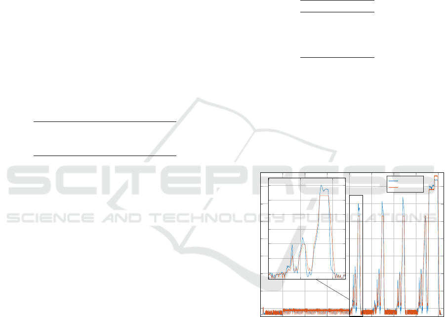
5.1 Regression of the Drum Speed
Results regarding the drum speed estimation are re-
ported in terms of RMSE in table 4. In accordance
Table 4: Results obtained for drum speed regression using
a different number of hidden units.
n
h
RMSE
2 50.78 rpm
10 41.38 rpm
40 33.87 rpm
50 38.60 rpm
with the outcome of the Bayesian optimization, the
best result is obtained using 40 hidden units. A lower
state dimension results in a network that is not com-
plex enough to model the time sequence, hence the
RMSE increases. On the contrary, using a model
which is too complex for this task leads to overfit-
ting, hence to worse results. In Figure 2 an example
of time domain result of the normalized drum speed
estimation is shown.
0 0.2 0.4
0.6
0.8 1 1.2 1.4
1.6
·10
4
0
1
2
3
4
5
6
7
Sample [-]
Normalized Drum Speed [-]
Predicted
Test
8,000
8,500
9,000
0
1
2
3
4
5
6
Figure 2: Time domain result of normalized drum speed
estimation. For clarity’s sake, part of the plot has been
zoomed on the left.
5.2 Classification of Loads
Results for each load are reported in Table 5.
The performances obtained for the heater status
classification are good using both deep learning tools.
This is due to the fact that the heater, when active,
draws from the grid a large amount of energy. Hence,
the real part of the first current harmonic increases
very much when this load is active, thus making the
status detection easier for the net. Similar results are
Loads Estimation using Deep Learning Techniques in Consumer Washing Machines
431

Table 5: Results obtained for load classification using LSTM and CNN.
Network Heater Drain Pump Electrovalves
LSTM
F1 class ON 99.82% 97.44% 37.61%
F1 class OFF 99.68% 99.54% 87.81%
CNN
F1 class ON 99.72% 98.57% 98.39%
F1 class OFF 99.95% 99.75% 99.87%
obtained for the drain pump. This load is quite easy
to detect and hence both the deep learning approaches
provide good results. The same cannot be said for
electrovalves. Regarding this load, it is clear that
CNNs outperform LSTMs.
6 CONCLUSIONS
In this work two different problems have been faced:
the drum speed estimation of a washing machine and
the activation status classification of different loads of
the same appliance. The first has been solved training
an LSTM network that estimates the speed at each
time instant. Results on the test set prove that good
performances can be achieved using this network, es-
pecially if the state dimension of the network is set
solving an optimization problem.
As for the second problem, two different ap-
proaches have been tested. The first consisted in
training an LSTM network (with an optimal number
of hidden units) whereas the second makes use of
CNNs. Good results have been achieved using both
the networks for two out of three loads (heater and
drain pump). Conversely, it is clear that using only
a weighted classification layer in the electrovalves-
status classification, is not enough to cope with class
unbalance, thus using CNNs leads to much better re-
sults. Hence, even though LSTMs are easier to train
and test (since the only preprocessing operation re-
quired is the normalization), CNNs will be preferred
since perform better in classifying all the loads.
REFERENCES
Alasalmi, T., Suutala, J., and R
¨
oning, J. (2012). Real-
time non-intrusive appliance load monitor. In Inter-
national conference on Smart grids and Green IT Sys-
tems, pages 203–208.
Batista, G. E., Prati, R. C., and Monard, M. C. (2004). A
study of the behavior of several methods for balancing
machine learning training data. ACM SIGKDD explo-
rations newsletter, 6(1):20–29.
Buda, M., Maki, A., and Mazurowski, M. A. (2018). A
systematic study of the class imbalance problem in
convolutional neural networks. Neural Networks,
106:249–259.
Djordjevic, S. and Simic, M. (2018). Nonintrusive identifi-
cation of residential appliances using harmonic anal-
ysis. Turkish Journal of Electrical Engineering and
Computer Sciences, 26.
Glorot, X., Bordes, A., and Bengio, Y. (2011). Deep sparse
rectifier neural networks. In Proceedings of the four-
teenth international conference on artificial intelli-
gence and statistics, pages 315–323.
Goodfellow, I., Bengio, Y., and Courville, A. (2016). Deep
learning. MIT press.
Grangier, D., Bottou, L., and Collobert, R. (2009). Deep
convolutional networks for scene parsing. In ICML
2009 Deep Learning Workshop, volume 3, page 109.
Citeseer.
Hannun, A. Y., Rajpurkar, P., Haghpanahi, M., Tison, G. H.,
Bourn, C., Turakhia, M. P., and Ng, A. Y. (2019).
Cardiologist-level arrhythmia detection and classifi-
cation in ambulatory electrocardiograms using a deep
neural network. Nature medicine, 25(1):65.
Hochreiter, S. and Schmidhuber, J. (1997). Long short-term
memory. Neural computation, 9(8):1735–1780.
Huang, X., Yin, B., Zhang, R., and Wei, Z. (2019). Study
of steady-state feature extraction algorithm based on
emd. In IOP Conference Series: Materials Science
and Engineering, volume 490, page 062036. IOP Pub-
lishing.
Jeni, L. A., Cohn, J. F., and De La Torre, F. (2013). Fac-
ing imbalanced data–recommendations for the use of
performance metrics. In 2013 Humaine association
conference on affective computing and intelligent in-
teraction, pages 245–251. IEEE.
Kim, J., Le, T.-T.-H., and Kim, H. (2017). Nonintrusive
load monitoring based on advanced deep learning and
novel signature. Computational intelligence and neu-
roscience, 2017.
Krizhevsky, A., Sutskever, I., and Hinton, G. E. (2012). Im-
agenet classification with deep convolutional neural
networks. In Advances in neural information process-
ing systems, pages 1097–1105.
Maitre, J., Glon, G., Gaboury, S., Bouchard, B., and
Bouzouane, A. (2015). Efficient appliances recog-
nition in smart homes based on active and reactive
power, fast fourier transform and decision trees. In
Workshops at the Twenty-Ninth AAAI Conference on
Artificial Intelligence.
Mocanu, E., Nguyen, P. H., Gibescu, M., and Kling, W. L.
(2016). Deep learning for estimating building energy
consumption. Sustainable Energy, Grids and Net-
works, 6:91–99.
Susto, G. A., Zambonin, G., Altinier, F., Pesavento, E., and
Beghi, A. (2018). A soft sensing approach for clothes
load estimation in consumer washing machines. In
2018 IEEE Conference on Control Technology and
Applications (CCTA), pages 1252–1257. IEEE.
ICPRAM 2020 - 9th International Conference on Pattern Recognition Applications and Methods
432