Estimation of Muscle Fascicle Orientation in Ultrasonic Images

Regina Pohle-Fr

ohlich

, Christoph Dalitz

1 a

, Charlotte Richter

2,3

Tobias Hahnen

, Benjamin St

audle

2,3

and Kirsten Albracht

2,3 b

Institute for Pattern Recognition, Niederrhein University of Applied Sciences, Reinarzstr. 49, Krefeld, Germany

Institute of Biomechanics and Orthopaedics, German Sport University Cologne, Cologne, Germany

Department of Medical Engineering and Technomathematics, Aachen University of Applied Science, Germany

Keywords:

Texture Direction, Orientation Angle, Gray Level Cooccurrence, Vesselness Filter, Projection Proﬁle, Radon

Transform.

Abstract:

We compare four different algorithms for automatically estimating the muscle fascicle angle from ultrasonic

images: the vesselness ﬁlter, the Radon transform, the projection proﬁle method and the gray level cooccurence

matrix (GLCM). The algorithm results are compared to ground truth data generated by three different experts

on 425 image frames from two videos recorded during different types of motion. The best agreement with

the ground truth data was achieved by a combination of pre-processing with a vesselness ﬁlter and measuring

the angle with the projection proﬁle method. The robustness of the estimation is increased by applying the

algorithms to subregions with high gradients and performing a LOESS ﬁt through these estimates.

1 INTRODUCTION

Human movement results from a coordinated acti-

vation of the skeletal muscles. The muscle fascicle

length and their change in length is critical for the

force and efﬁciency of the muscle. It is thus necessary

to measure fascicle length, which is usually done from

ultrasonic images (Fukunaga et al., 1997; Fukunaga

et al., 2001; Zhou and Zheng, 2012). An example

of a B-mode ultrasound image of the muscle gastroc-

nemius medialis recorded with an ALOKA Prosound

α7 can be seen in Fig. 1: the fascicles are spanned

between the two aponeuroses.

As the fascicles are interrupted by noise and rarely

are captured in their full length by the imaging pro-

cess, their length must be computed from three dif-

ferent auxiliary observables: the position of the two

aponeuroses and the fascicle orientation angle (pen-

nation). Throughout the present paper, we make the

simplifying assumption that both aponeuroses can be

approximated by straight lines. The fascicle length

can then be computed from the pennation angle at dif-

ferent positions on these lines. We thus only concen-

trate on the problem of ﬁnding the aponeuroses and

estimating the pennation angle.

https://orcid.org/0000-0002-7004-5584

https://orcid.org/0000-0002-4271-2511

When the imaging is done while the muscle is

in motion, the image quality can deteriorate due

to variation of transducer skin contact and position

(Aggeloussis et al., 2010). If the fascicle length or

orientation estimation is not done manually, but semi-

automatic or even fully automatic, this requires thus

robust image processing methods for possibly noisy

videos.

According to (Yuan et al., 2020), algorithms for

automatically estimating the fascicle orientation can

be divided into three different approaches. In the ﬁrst

category, the tracking is semi-automatic by follow-

ing a manually marked indicidual ﬁbers in subsequent

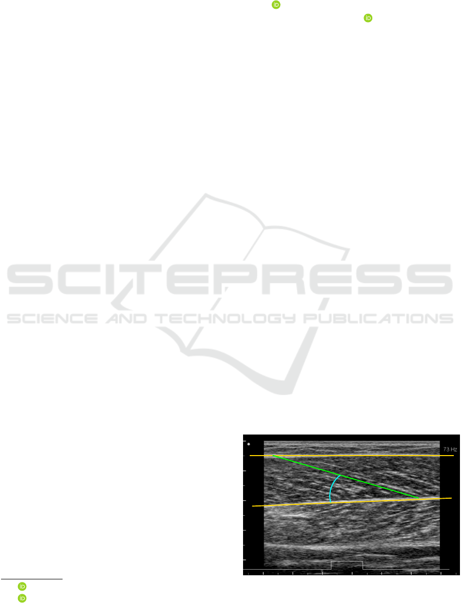
superficial aponeurosis

deep aponeurosis

pennation

angle

fascicle length

Figure 1: Annotated example of an ultrasonic image of the

muscle gastrocnemius medialis.

Pohle-Fröhlich, R., Dalitz, C., Richter, C., Hahnen, T., Stäudle, B. and Albracht, K.

Estimation of Muscle Fascicle Orientation in Ultrasonic Images.

DOI: 10.5220/0008933900790086

In Proceedings of the 15th International Joint Conference on Computer Vision, Imaging and Computer Graphics Theory and Applications (VISIGRAPP 2020) - Volume 5: VISAPP, pages

79-86

ISBN: 978-989-758-402-2; ISSN: 2184-4321

frames. This can be done, for example by calculating

the optical ﬂow, like in the UltraTrack software (Far-

ris and Lichtwark, 2016). A disadvantage of these

methods is the cumulative error, which requires man-

ual correction after several frames. In addition, mis-

alignments may result due to signiﬁcant changes in

the appearance and intensity of the structures between

successive frames. These problems occur particularly

with large displacement ﬁelds due to fast motion and

insufﬁcient sampling rates of most currently available

commercial devices.

Methods based on texture feature detection form

the second category, which includes Hough transform

(Zhou and Zheng, 2008), Radon transform (Zhao and

Zhang, 2011), or vesselness ﬁlter (Rana et al., 2009).

The disadvantage of these methods is that the result

of the angle estimation may be distorted by speckle

noise and intramuscular blood vessels, which modify

the characteristics of the muscle fascicles.

The third category includes deep learning ap-

proaches. Cunningham proposed deep residual (Cun-

ningham et al., 2017) and convolution neural net-

works (Cunningham et al., 2018) to estimate the mus-

cle fascicle orientation. One problem with using deep

learning methods is that they require a large amount

of manually measured image data to achieve good re-

sults. Another difﬁculty is the dependence of the im-

age acquisition and the image distortions on the ul-

trasound transducer, so that adjusted data sets are re-

quired.

In the present article, we compare two estab-

lished methods from the literature with two new ap-

proaches to determine the orientation of textures. As

established methods, we consider vesselness ﬁltering

(Rana et al., 2009) and Radon transform (Zhao and

Zhang, 2011). We compare these with the very re-

cently proposed gray value cooccurence matrix based

texture orientation estimation (Zheng et al., 2018) and

the calculation of the angle using the projection pro-

ﬁle (Dalitz et al., 2008). The latter method has been

used for some time in document image analysis for

estimating the rotation of binary documents. Here we

demonstrate that it can be used for gray level images,

too.

In order to evaluate the quality of the different al-

gorithms, we have compared their results with man-

ual estimations of the pennation angle by different ex-

pert observers. As evaluation criteria, we utilized the

intra-class correlation and the mean absolute percent-

age with respect to the inter-observer average, and the

percentage of results within the inter-observer range.

This article is organized as follows: in section 2 &

3 we describe the implemented algorithms, section 4

describes the evaluation method, section 5 discusses

the results and compares the algorithm performances,

and in section 6 we draw some conclusions and give

recommendations for a practical utilization of the al-

gorithms.

2 REGION OF INTEREST

EXTRACTION

To determine the region of interest (ROI), each video

frame is evaluated separately. Firstly, the two black

areas (see Fig.1) are removed. Then, for a reinforce-

ment of the aponeuroses a vesselness ﬁltering (see

section 3.2) is carried out. Then, Otsu’s threshold-

ing method is used generate a binary image of the

ﬁltered image. In the result, the two largest seg-

ments which correspond to the two aponeuroses are

selected. Straight lines are ﬁtted to the lower segment

border of the superﬁcial aponeurosis and to the up-

per segment border of the deep aponeurosis using the

least squares method. The height of the ROI resulted

from the difference between the smallest y-value of

the lower aponeurosis minus 10 pixels and the largest

y-value of the upper aponeurosis plus 10 pixels. The

width of the ROI is calculated from the width of the

image minus a safety area of 10 pixels to the left and

right borders. This ensures that the ROI is always po-

sitioned within the muscle. As the noise level or the

orientation angle may vary over the entire ROI, we

additionally subdivided the entire region horizontally

into eight overlapping subregions. For a fully auto-

mated process, it would be necessary to automatically

pick the subregion with the “best” image quality. To

characterize this quality, we have computed, for every

subregion, the gray value variance as a measure for

contrast, the mean gradient value and the maximum

value of the histogram of the gradients as measures

for edge sharpness.

3 FASCICLE DIRECTION

ESTIMATION

For the determination of the ﬁber orientation we used

different methods, which are described in the follow-

ing. These methods were either applied directly to the

ROI or a pre-processing step was used for fascicle en-

hancement. For pre-processing, a Vesselness ﬁlter or

Radon transformation was optionally applied for im-

age enhancement. Tbl. 1 shows the investigated com-

binations for pre-processing and fascicle orientation

estimation.

VISAPP 2020 - 15th International Conference on Computer Vision Theory and Applications

Table 1: Tested combinations for pre-processing and fasci-

cle orientation estimation. “Frangi” denotes the vesselness

ﬁlter.

orientation pre-processing

estimation none Frangi Radon

Frangi - x -

Radon - - x

GLCM x x x

projections x x x

3.1 Radon Transform

The Radon transformation determines the line inte-

gral of the function f (x,y) along all straight lines of

the xy plane. For each of these straight lines one can

consider the Radon transform R as a projection of the

function f (x,y) onto a straight line perpendicular to

it. For this reason it was used by (Zhao and Zhang,

2011), (Yuan et al., 2020) to determine the orientation

of the muscle ﬁbers in ultrasound images. It should

be noted that the radon transformation cannot only be

used for direct angle estimation, but also merely as a

pre-processing operation to reinforce fascicles. Such

a pre-processed image E with an enhancement of the

linear structures in the initial image I is achieved by

applying the following equation:

E = R

−1

(sign(R(I)) · R(I)

) (1)

where R is the Radon transform and R

−1

is the inverse

Radon transform. The result of the Radon transform

based enhancement is shown in Fig. 2(c). The angle

of the fascicle orientation resulted from the position of

(a) raw data

(b) vesselnes ﬁlter (Frangi)

Figure 2: Effect of ﬁltering with the vesselness ﬁlter or

the Radon transform on an image recorded during running

movement.

the maximum of the radon transformed. In our tests,

we calculated the radon transformation only for an an-

gular range of 15 to 70 degrees in which the actual

values vary to exclude errors due to the orientation of

the speckle pattern.

3.2 Vesselness Filter

Muscle fascicles appear in ultrasound images as

vessel-like tubular structures, so that in (Rana et al.,

2009) the multiscale vesselness ﬁlter developed by

Frangi (Frangi et al., 1998) was used to enhance them.

In the ﬁrst step of this ﬁlter, images are convolved

with Gaussian kernels. Then the Hessian matrix of

these convolved images is computed. Their eigen-

values provide information related to the direction of

line-like structures. The eigenvector in the direction

of the smallest eigenvalue yields the orientation angle

at the respective pixel position. For our tests we used

the implementation in libfrangi

whereby we only al-

lowed angles within our chosen range of 15 to 70 de-

grees in order to suppress responses from dominating

horizontal or vertical structures. All values outside

this range were set to zero in the result image. To

estimate a total orientation angle from all the local

angles estimated at non-zero pixels, we estimated the

angle distribution with a kernel density estimator with

“Silverman’s rule of thumb” (Sheather, 2004) and de-

termined the angle maximizing this density.

Like the radon transform, the vesselness ﬁlter can

alternatively also merely be used as a pre-processing

operation for enhancing fascicle structures. An exam-

ple is shown in Fig. 2(b).

3.3 Projection Proﬁle

The projection proﬁle method (Dalitz et al., 2008) es-

timates the orientation angle α as the angle with the

highest variation of the skewed projection proﬁle

(y) =

x=∞

∑

x=−∞

f (x cos α − y sinα,x sin α + ycos α)

(2)

where f (x, y) is the gray value of the ultrasound image

at position (round(x),round(y)) and zero outside the

image. The variation of this proﬁle is deﬁned as

V (α) =

y=∞

∑

y=−∞

(y + 1) − h

(y)]

(3)

In our implementation we calculate the variation for

an angle range from 15 to 70 degrees with a step width

of 0.5 degrees, which corresponds to the possible an-

gles occurring for our recording conditions. Then we

https://github.com/ntnu-bioopt/libfrangi

Estimation of Muscle Fascicle Orientation in Ultrasonic Images

select the angle corresponding to the highest varia-

tion.

3.4 Graylevel Cooccurence

The gray level cooccurence matrix (GLCM) repre-

sents an estimate of the probability that a pixel at

position (x, y) in an image with a graylevel g

has a

graylevel g

at position (x + dx,y + dx ). The GLCM

has a size of g

max

×g

max

, whereby g

max

−1 is the max-

imum of the gray levels in the image. If arbitrary rela-

tive positions are used to calculate the GLCM, the tex-

ture orientation can be estimated. Zheng (Zheng et al.,

2018) applied this method to evaluate SAR images of

the sea surface. For the calculation of the GLCM, we

utilized in the method that Zheng et al. called “scheme

1”. If the shift vector (dx,dy) = (r · cosα,r · sinα)

corresponds with the texture orientation, the diagonal

elements of the GLCM attain high values. For the es-

timation of the fascicle orientation, we apply the crite-

rion suggested in (Zheng et al., 2018), i.e., the degree

of concentration C of larger elements of the GLCM

with respect to the diagonal line:

C(r, α) =

max

−1

∑

m=0

max

−1

∑

n=0

(m − n)

· GLCM(m,n; r, α)

(4)

The weight (m − n)

, which increases with increasing

distance of the matrix element from the diagonal, re-

sults in smaller values for images with a strong line

structure if the angle α corresponds to the orientation

of this structure. In our experiments we used a maxi-

mum r of 40 and an angle range of 15 to 70 degrees.

The used angle corresponded to the angle α with the

lowest concentration value.

3.5 Local Regression

Due to the noisy nature of the images, the angle es-

timate can ﬂuctuate considerably between adjacent

frames and subregions. It is thus natural to seek a

more robust angle estimate by means of local regres-

sion. To this end, we optionally apply Cleveland

& Devin’s LOESS method (Cleveland and Devlin,

1988), which is a distance weighted least squares ﬁt

over the k nearest neighbors with weight

(z) =

(



1 − (z/h)



for |z| < h

0 otherwise

(5)

where h is the distance to the k-th nearest neighbor.

In our case, the predictor is the frame number and the

dependent variable is the pennation angle.

A B C all

0 2 4 6 8

expert

spread in degrees

Figure 3: Spread per frame of the pennation angle estimates

of the three experts.

4 EVALUATION METHOD

In order to evaluate and compare the different algo-

rithms, we have asked three different experts to manu-

ally draw the aponeurosis and fascicle orientation into

ultrasonic images with the user interface of the Ultra-

Track software (Cronin et al., 2011). The images were

taken from two different videos, which were recorded

each with an ALOKA Prosound α7 for ﬁve consec-

utive stance phases (touchdown to toe-off) of the left

foot during walking (video “W”) and running (video

“R”). This resulted in a total of 425 different frames.

The muscle fascicles in the R video were less clearly

visible tan in the W video due to the shakier trans-

ducer skin contact during running.

Each frame was examined three times by every ex-

pert, but on different days. We thus had nine differ-

ent manually estimated angles for each frame. This

was done to estimate the accuracy of the expert opin-

ion. The intra-class correlation ICC3 (Shrout and

Fleiss, 1979) between the experts’ angle estimations

was 0.97, which means that there was good agree-

ment among the experts which angles were higher and

which were lower. On the other hand, the average an-

gle spread per frame was 1.9

◦

for expert A, 1.7

◦

for

expert B, 1.1

◦

for expert C, and 3.2

◦

over all experts.

Box-Plots for the spread distribution can be seen in

Fig. 3. The spread between experts was thus consider-

ably greater than within each expert, and we conclude

that we cannot expect an algorithm to estimate the an-

gle with an accuracy greater than about two degrees.

Part of the inter- and intra-observer variation can

be explained by varying fascicle orientations for dif-

ferent image regions. We therefore split the region

of interest into eight slightly overlapping subregions

and ran the algorithms on each subregion plus on the

VISAPP 2020 - 15th International Conference on Computer Vision Theory and Applications

190 200 210 220 230 240

20 25 30 35

frame

angle

projection

GLCM

Frangi

Radon

(a) walking (video W)

270 275 280 285 290 295

20 25 30 35 40 45

frame

angle

projection

GLCM

Frangi

Radon

(b) running (video R)

Figure 4: Angle estimations of the different algorithms applied to the entire region of interest for two typical steps of motion.

The gray area is the inter-observer range.

entire region. For each algorithm, we then measured

the following performance indicators for each of these

nine regions:

• the intra-class correlation (ICC3) with the inter-

observer average; this measures how well the es-

timated angles follow the curve shape

• the mean absolute error (MAE) with respect to the

inter-observer average; this measures the overall

error in the estimation in degrees

• the percentage of values inside the inter-observer

range (hit)

5 RESULTS

As the pennation angle is deﬁned as the angle between

the deep aponeurosis and the muscle fascicles, there

are two possible sources of error for its estimation:

errors in the estimation of the aponeurosis’ slope, and

in the estimation of the fascicle orientation. We there-

fore ﬁrst evaluated the aponeurosis estimation, and

then the estimation of the pennation angle. Moreover,

to derive recommendations for pre-processing ﬁlter-

ing, we report results for the different combinations of

pre-processing and estimation algorithms listed above

in Tbl. 1.

5.1 Aponeurosis Slope

In video “R”, the deep aponeurosis was very close to a

straight line, and algorithm and expert opinion about

its slope angle was in good agreement: ICC3=0.926,

MAE=0.286

◦

, hit=71%.

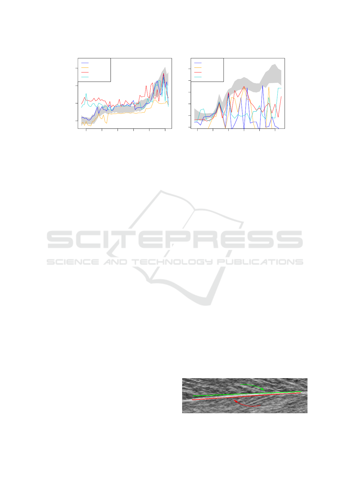
In video “W”, the deep aponeurosis was curved

slightly (see Fig. 5) and the experts tended to estimate

the slope at the right end, whilst the algorithm com-

puted an average slope over its entire width. This had

the effect that the automatic estimate of its slope an-

gle was on average one degree greater than the expert

opinion: ICC3=0.764, MAE=1.081

◦

, hit=4%.

As the decision at which position the tangential

angle of the aponeurosis is measured is somewhat ar-

bitrary, we conclude that the aponeurosis slope angle

is estimated by our algorithm within the possible ac-

curacy. The difference in slope estimation has no ef-

fect for video “R”, but for video “W” it leads to a

systematic difference of about one degree for the pen-

nation angle, i.e., the automatically estimated penna-

tion angle in video “W” should be about one degree

greater than the manually estimated angle.

5.2 Pennation Angle

For the pennation angle, we have evaluated two dif-

ferent approaches to its estimation. The ﬁrst approach

models the angle as a single texture feature over the

entire ROI, whilst the second approach models it as

locally and statistically varying and applies a LOESS

ﬁt over subregions of neighboring frames.

5.2.1 Entire Region

It turned out that the results were very different for

the two videos: for all algorithms, all performance in-

dices were considerably better on the less noisy video

manual

algorithm

Figure 5: The aponeurosis curvature in video “W” leads to

a small difference in the aponeurosis slope estimation.

Estimation of Muscle Fascicle Orientation in Ultrasonic Images

190 200 210 220 230 240

20 25 30 35

frame

angle

projection

GLCM

Frangi

Radon

(a) walking (video W)

270 275 280 285 290 295

20 25 30 35 40 45

frame

angle

projection

GLCM

Frangi

Radon

(b) running (video R)

Figure 6: Angle estimations of the different algorithms applied to the three regions with the highest mean gradient and with

LOESS ﬁtting for two typical steps of motion. For video R, the projection method was so far off that its values do not fall into

the displayed angle range. The gray area is the inter-observer range.

Table 2: Angle estimation performance indices of the dif-

ferent algorithms applied to the entire region of interest.

algorithm video ICC3 MAE hit

projection W 0.871 1.231

◦

58%

R -0.003 9.335

◦

35%

GLCM W 0.784 2.221

◦

33%

R 0.180 10.437

◦

10%

Frangi W 0.552 2.998

◦

17%

R 0.524 5.493

◦

33%

Radon W 0.540 2.309

◦

42%

R 0.430 6.506

◦

32%

“W” (see Tbl. 2). The best performing algorithm

was the projection proﬁle method, followed by the

GLCM. As can be seen in Fig. 4(a), the angles es-

timated by the other two algorithm follow the curve

shape with lesser agreement, which corresponds to

poorer ICC3 values in Tbl. 2.

For video “R”, however, neither of the algorithms

yielded satisfying results, as can be concluded from

the poor performance indices in Tbl. 2 and the random

ﬂuctuations of the estimated angles inf Fig. 4(b).

5.2.2 LOESS Fit Over Subregions

To obtain a more robust angle estimator, we calcu-

lated the estimates for eight subregions, selected the

“best” three subregions per frame and made a LOESS

ﬁt over these subregions including the eight neighbor-

ing frames. As our predictor was the frame number,

the distance z in Eq. (5) was measured in frame num-

bers and the number of neighbors was k = 27.

This raises the question, how the “best” subre-

gions are selected for each frame. A human expert

would focus on a region in which the fascicles are

clearly visible, i.e. a region with high contrast or sharp

edges. The three criteria listed in section 2 try to mea-

Table 3: Angle estimations of the different algorithms ap-

plied to the three regions with the highest mean gradient

and with LOESS ﬁtting.

algorithm

video ICC3 MAE hit

projection W 0.975 0.548

◦

86%

R 0.096 12.895

◦

GLCM W 0.926 1.567

◦

27%

R 0.848 4.122

◦

29%

Frangi W 0.733 1.704

◦

49%

R 0.635 6.688

◦

14%

Radon W 0.804 2.007

◦

41%

R 0.868 3.357

◦

36%

sure this property. It turned out that the actual crite-

rion has a smaller effect than the choice of algorithm.

We thus present the results that use the highest mean

gradient as a criterion for the “best” subregions; the

results for the other criteria are similar.

As can be seen from Tbl. 3, the LOESS ﬁt

improves the performance indices in almost all

cases. One notable exception is the projection proﬁle

method for video “R”: in this case the angle estimates

were so far off that they even fell outside the range

of Fig. 6(b), although this algorithm performed best

on video “W”. We thus conclude that the projection

proﬁle method should be used in combination with a

pre-processing ﬁlter because it is not robust with re-

spect to high levels of noise.

5.3 Effect of Pre-processing

To see whether using the Radon transform or the ves-

selness ﬁlter (“Frangi”) as a pre-processing operation

improves the performance of the other algorithms, we

have ﬁrst applied these ﬁlters and then utilized the

same LOESS approach as in the preceding subsec-

tion. As can be seen from Tbl. 4, this did not improve

VISAPP 2020 - 15th International Conference on Computer Vision Theory and Applications

190 200 210 220 230 240

20 25 30 35

frame

angle

projection (Frangi)

projection (Radon)

GLCM (Frangi)

GLCM (Radon)

(a) walking (video W)

270 275 280 285 290 295

20 25 30 35 40 45

frame

angle

projection (Frangi)

projection (Radon)

GLCM (Frangi)

GLCM (Radon)

(b) running (video R)

Figure 7: Effect of the pre-processing ﬁlters (in parentheses) on angle estimations applied to the three regions with the

highest mean gradient and with LOESS ﬁtting for two typical steps of motion. For video R, the GLCM method with Frangi

(vesselness ﬁlter) pre-processing was so far off that its values do not fall into the displayed angle range. The gray area is the

inter-observer range.

Table 4: Angle estimations after pre-processing applied to

the three regions with the highest mean gradient and with

LOESS ﬁtting.

algorithm video ICC3 MAE hit

projection W 0.946 1.962

◦

25%

(with Frangi) R 0.946 1.871

◦

62%

projection W 0.755 2.231

◦

31%

(with Radon) R 0.665 4.500

◦

29%

GLCM W 0.914 2.408

◦

21%

(with Frangi) R 0.058 39.699

◦

GLCM W 0.718 2.912

◦

20%

(with Radon) R 0.695 4.316

◦

23%

the performance of the GLCM with respect to Tbl. 3,

but for the projection proﬁle method, pre-processing

with a vesselness ﬁlter seriously improved the results

for video “R”. Overall, the combination “vesselness

ﬁlter and projection proﬁle method” was the best per-

forming algorithm, followed secondly by the GLCM

without pre-processing.

6 CONCLUSIONS

Based upon our experimental evaluation, we recom-

mend two possible algorithms for estimating the pen-

nation angle in ultrasonic images of muscles. The best

performing algorithm was a combination of the ves-

selness ﬁlter as a pre-processing operation with the

projection proﬁle method for angle estimation. This

algorithm achieved an intra-class correlation close to

one and had a mean average error less than two de-

grees. The second best algorithm was based on the

gray level cooccurance matrix (GLCM).

Both the robustness and accuracy of the angle esti-

mates are considerably improved by a LOESS ﬁt over

neighboring frames and the subregions with the best

visible edges. In our study, we have selected these

regions automatically on basis of the mean absolute

value of the gradient within the subregion.

In practice, if a semi-automatic processing is pos-

sible, the region selection process could alternatively

done by an expert user. This would also have the ben-

eﬁt that the fascicle length computation can be based

on the selected region. This is of relevance, because

the fascicle length is not well deﬁned if the superﬁcial

and the deep aponeuroses are not parallel. In this case,

a hint by an expert user is necessary in any case where

to set an anchor point of the line used for computing

the fascicle length, which could be chosen, e.g., as the

mid point of the user selected region.

ACKNOWLEDGMENTS

Parts of this study were ﬁnancially supported by the

German Federal Ministry of Economic Affairs and

Energy under grant no. 50WB1728.

REFERENCES

Aggeloussis, N., Giannakou, E., Albracht, K., and Aram-

patzis, A. (2010). Reproducibility of fascicle length

and pennation angle of gastrocnemius medialis in hu-

man gait in vivo. Gait & posture, 31(1):73–77.

Cleveland, W. S. and Devlin, S. J. (1988). Locally weighted

regression: an approach to regression analysis by local

ﬁtting. Journal of the American statistical association,

83(403):596–610.

Estimation of Muscle Fascicle Orientation in Ultrasonic Images

Cronin, N. J., Carty, C. P., Barrett, R. S., and Lichtwark, G.

(2011). Automatic tracking of medial gastrocnemius

fascicle length during human locomotion. Journal of

Applied Physiology, 111(5):1491–1496.

Cunningham, R., Harding, P., and Loram, I. (2017). Deep

residual networks for quantiﬁcation of muscle ﬁber

orientation and curvature from ultrasound images. In

Annual Conference on Medical Image Understanding

and Analysis, pages 63–73. Springer.

Cunningham, R., S

anchez, M., May, G., and Loram, I.

(2018). Estimating full regional skeletal muscle ﬁ-

bre orientation from B-mode ultrasound images us-

ing convolutional, residual, and deconvolutional neu-

ral networks. Journal of Imaging, 4(2):29.

Dalitz, C., Michalakis, G. K., and Pranzas, C. (2008). Opti-

cal recognition of psaltic byzantine chant notation. In-

ternational Journal of Document Analysis and Recog-

nition (IJDAR), 11(3):143–158.

Farris, D. J. and Lichtwark, G. A. (2016). UltraTrack: Soft-

ware for semi-automated tracking of muscle fascicles

in sequences of B-mode ultrasound images. Computer

Methods and Programs in Biomedicine, 128:111–118.

Frangi, A. F., Niessen, W. J., Vincken, K. L., and Viergever,

M. A. (1998). Multiscale vessel enhancement ﬁlter-

ing. In International conference on medical image

computing and computer-assisted intervention, pages

130–137.

Fukunaga, T., Ichinose, Y., Ito, M., Kawakami, Y., and

Fukashiro, S. (1997). Determination of fascicle length

and pennation in a contracting human muscle in vivo.

Journal of Applied Physiology, 82(1):354–358.

Fukunaga, T., Kubo, K., Kawakami, Y., Fukashiro, S.,

Kanehisa, H., and Maganaris, C. N. (2001). In vivo

behaviour of human muscle tendon during walking.

Proceedings of the Royal Society of London. Series B:

Biological Sciences, 268(1464):229–233.

Rana, M., Hamarneh, G., and Wakeling, J. M. (2009). Au-

tomated tracking of muscle fascicle orientation in B-

mode ultrasound images. Journal of biomechanics,

42(13):2068–2073.

Sheather, S. J. (2004). Density estimation. Statistical sci-

ence, 19(4):588–597.

Shrout, P. E. and Fleiss, J. L. (1979). Intraclass correla-

tions: uses in assessing rater reliability. Psychological

bulletin, 86(2):420.

Yuan, C., Chen, Z., Wang, M., Zhang, J., Sun, K., and Zhou,

Y. (2020). Dynamic measurement of pennation angle

of gastrocnemius muscles obtained from ultrasound

images based on gradient radon transform. Biomed-

ical Signal Processing and Control, 55:101604.

Zhao, H. and Zhang, L. (2011). Automatic tracking of

muscle fascicles in ultrasound images using localized

radon transform. IEEE Transactions on Biomedical

Engineering, 58(7):2094–2101.

Zheng, G., Li, X., Zhou, L., Yang, J., Ren, L., Chen, P.,

Zhang, H., and Lou, X. (2018). Development of a

gray-level co-occurrence matrix-based texture orien-

tation estimation method and its application in sea

surface wind direction retrieval from SAR imagery.

IEEE Transactions on Geoscience and Remote Sens-

ing, 56(9):5244–5260.

Zhou, G. and Zheng, Y. (2012). Human motion analysis

with ultrasound and sonomyography. In 2012 Annual

International Conference of the IEEE Engineering in

Medicine and Biology Society, pages 6479–6482.

Zhou, Y. and Zheng, Y.-P. (2008). Estimation of muscle

ﬁber orientation in ultrasound images using revoting

Hough transform (RVHT). Ultrasound in medicine &

biology, 34(9):1474–1481.

VISAPP 2020 - 15th International Conference on Computer Vision Theory and Applications