Pre- and Post-processing Strategies for Generic Slice-wise

Segmentation of Tomographic 3D Datasets Utilizing U-Net Deep

Learning Models Trained for Specific Diagnostic Domains

Gerald A. Zwettler

1,2

, Werner Backfrieder

and David R. Holmes III

Biomedical Analytics and Computational Engineering Lab, Department of Physiology and Biomedical Engineering,

Mayo Clinic College of Medicine, 200 First St. SW, 55905 Rochester, MN, U.S.A.

Research Group Advanced Information Systems and Technology (AIST), Department of Software Engineering,

University of Applied Sciences Upper Austria, Softwarepark 11, 4232 Hagenberg, Austria

Medical Informatics, Department of Software Engineering, University of Applied Sciences Upper Austria,

Softwarepark 11, 4232 Hagenberg, Austria

Keywords: Deep Learning, U-Net, Model-based Segmentation in Medicine, Computed Tomography.

Abstract: An automated and generally applicable method for segmentation is still in focus of medical image processing

research. Since a few years artificial inteligence methods show promising results, especially with widely

available scalable Deep Learning libraries. In this work, a five layer hybrid U-net is developed for slice-by-

slice segmentation of liver data sets. Training data is taken from the Medical Segmentation Decathlon

database, providing 131 fully segmented volumes. A slice-oriented segmentation model is implemented

utilizing deep learning algorithms with adaptions for variable parenchyma shape along the stacking direction

and similarities between adjacent slices. Both are transformed for coronal and sagittal views. The

implementation is on a GPU rack with TensorFlow and Keras. For a quantitative measure of segmentation

accuracy, standardized volume and surface metrics are used. Results DSC=97.59, JI=95.29 and NSD=99.37

show proper segmentation comparable to 3D U-Nets and other state of the art. The development of a 2D-slice

oriented segmentation is justified by short training time and less complexity and therefore massively reduced

memory consumption. This work manifests the high potential of AI methods for general use in medical

segmentation as fully- or semi-automated tool supervised by the expert user.

1 INTRODUCTION

Automated and precise segmentation of anatomical

structures for computer-assisted diagnostics is still

field of ongoing research. Only for particular domains,

off-the-shelf applications are available (Christensen

and Wake, 2018) but generally computer-aided

diagnostic is achieved in a user-centric process

utilizing frameworks providing tools for semi-

automated processing (Strakos et al. 2015). The

manual processing of the datasets thereby necessitates

a lot of experience in both, the technical and the

medical domain and is exposed to subjective

processing, even if following a rather standardized

segmentation process (Zwettler et al. 2013).

1.1 Medical Background

The precise segmentation of specific anatomical

structures from 3D data forms the basis for quantita-

tive analysis in computer-assisted diagnostics. The

quantitation aspect is relevant for assessing disease

progression or general scoring (Aggarwal et al. 2011).

Based on segmented anatomical structures, the

visualization and inspection in 3D, as well as

utilization in AR and VR environments becomes

feasible. Segmentations are further relevant for surgery

planning, building up anatomical atlas models,

evaluating image acquisition protocols or as input data

for nowadays widely available 3D print (Squelch

2018).

1.2 Sate of the Art

Since the appearance of the first CT scanners, in the

early 1970s, intensive research in the field of medical

image processing targeting at fully automated

segmentation approaches has been initiated and is still

going on.

Zwettler, G., Backfrieder, W. and Holmes III, D.

Pre- and Post-processing Strategies for Generic Slice-wise Segmentation of Tomographic 3D Datasets Utilizing U-Net Deep Learning Models Trained for Speciﬁc Diagnostic Domains.

DOI: 10.5220/0008932100660078

In Proceedings of the 15th International Joint Conference on Computer Vision, Imaging and Computer Graphics Theory and Applications (VISIGRAPP 2020) - Volume 5: VISAPP, pages

66-78

ISBN: 978-989-758-402-2; ISSN: 2184-4321

A priori knowledge about the target shape, lead to

deformable models (McInerney and Terzopoulos

1996). With statistical shape (Cootes et al. 1992),

adaptive models are calculated from a large set of

reference datasets with corresponding reference

positions, thus representing the statistical shape

variability of the target anatomical structure in a

sophisticated way. Statistical Shape models allow for a

very compact representation of the target’s structure

due to PCA but the precise and generic determination

of corresponding landmarks is still unsolved and

necessitates specific approaches in particular

diagnostic domains. Incorporating the input dataset

intensity profiles besides shape, Active Appearance

Models (Cootes et al. 1998) can be trained for

automated segmentation in specific anatomical

domains but attracted interest and significance in a

non-diagnostic domain, namely human face

comparison and recognition.

In recent years, improvements in GPU speed,

massive efforts in AI research of large companies and

availability of machine learning frameworks such as

Tensorflow to the research community were the trigger

for significant improvements in Deep Learning and to

allow for technical implementation of some concepts,

since then only theoretically documented. The most

significant developments are thereby Feed Forward

networks with several hidden layers that are applicable

in many computer vision and also speech recognition

tasks. Nevertheless, Feed Forward networks are also

applied for medical multi-modal image fusion (Zhang

and Wang 2011). The concept of self-organizing

neural networks first introduced by Kohonen

(Kohonen 1995) for clustering in complex domains

was successfully applied to classification of renal

diseases too (Van Biesen 1998). With recurrent neural

networks and long/short-term-memories (LSTM)

(Hochreiter and Schmidhuber 1997) semantic

processing of input data sequences as relevant for OCR

and voice analysis, c.f. DeepVoice, became feasible

(Arik et al. 2017). One of the most significant

developments in Deep Learning in recent years are

convolutional neural networks, training kernels and

weights of multi-resolution filter pyramids and thus

clearly outperforming classic convolutional-layer

based approaches such as Haar Cascades (Viola and

Jones 2001). Some of the most relevant CNN

architectures are LeNet, AlexNet, GoogLeNet or

ResNet showing more than 1200 layer. New fields of

application opened generative adversial networks

(GAN) (Goodfellow et al. 2014). It is applied for

mimicking of natural data in domains as generating

paintings, hand written letters or medical data (Yi et al.

2019). The latter are used for automated liver

segmentation (Yang et al., 2017) or generation of test

data to prevent from over-fitting (Frid-Adar 2018).

1.3 Related Work

The U-Net architecture was initially developed for 2D

cell border classification (Ronneberg et al. 2014) but

soon transformed to processing 3D data too (Cicek et

al. 2016), applicable for brain tumor segmentation

(Amorim et al. 2017), liver segmentation (Meine et al.

2018) and various other medical diagnostic domains.

Recent notable advances in 3D U-Net architectures

are 3D dilated convolution kernels to significantly

speed-up the processing and allow for real-time

application (Chen et al. 2019) as well as generic

models for semantic segmentation on different

imaging modalities and anatomical structures (Huang

et al. 2019).

1.4 Generic Deep Learning Models

In this work, several approaches for utilizing

conventional U-Net architectures for slice-wise

processing of tomographic 3D datasets are presented.

Due to the utilized pre-processing strategy with ROI

selection and adjusting the intensity profile, the

approach evaluated on liver CT datasets is applicable

to different domains like lung, kidney or other

modalities such as brain MRI too.

Besides a sufficient amount of at least 100 volumes

along with precise reference segmentations, for the

generic segmentation approach no additional domain-

specific knowledge is incorporated.

Due to the slice-wise processing, important aspects

of the 3D dataset such as position within the patient get

lost. In this work several strategies are adressed and

evaluated to utilize positional information for the slice-

wise processing.

2 MATERIAL

For this research work, the liver datasets from the

Medical Segmentation Decathlon database (Simpson

et al., 2019) are utilized for training, validation and test.

The use of the database is restricted to the 131 liver

datasets that are provided together with reference

segmentations as ground truth. All 3D volumes are

available in NIFTI1 image format (DFWG, 2005), a

modification of the Analyze 7.5 format (BIR, 1986).

The medical image analysis software Analyze (Robb et

al. 1989) is utilized to convert the datasets from NIFTI1

to Analyze 7.5 and to perform the data preparation and

pre-processing subsequently described in section 2.2.

Pre- and Post-processing Strategies for Generic Slice-wise Segmentation of Tomographic 3D Datasets Utilizing U-Net Deep Learning

Models Trained for Speciﬁc Diagnostic Domains

2.1 Analytic Inspection of the

Task03_Liver Datasets

The 3D volumes are available as axial slices of matrix

size 512×512 with an average number of slices

sliceCnt

=447.62±275.25 [74;987]. The iso-spacing in

x/y-direction is given with µ

spacingXY

=0.793±.118

[.1557;1.000] and the inhomogeneous slice thickness

is described with µ

spacingXY

=1.506±1.177 [.699;5.000].

The intensities of the CT slices range between

intMIN

=-1103.26±204.93 [-2048;-1000] to

intMAX

=3334.70±3566.96 [1023;27748]. The vendor-

related suspicious low and high values are not further

addressed as they are out of the relevant intensity

context for the liver segmentation domain.

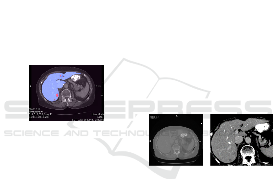
The reference segmentations provided for the liver

datasets represent a three-class non-overlapping

discrimination of the volume, namely background (0),

liver (1) and liver tumour (2) as shown in Fig.1 for slice

417 of dataset #0.

Figure 1: Med Decathlon slice 417 of liver dataset #0 with

parenchyma (blue) and the tumour (red) respectively.

2.2 Data Preparation and

Pre-processing

In this work a binary segmentation of the liver

parenchyma is the objective target. Thus, the ground

truth for liver and tumour areas are merged leading to

an encapsulated liver shape.

To balance the significant mismatch in slice

thicknesses, the z spacing is adjusted to the x/y inter-

slice spacing utilizing cubic interpolation for the

intensity dataset and shape interpolation (Rajagopalan

et al. 2003) for the binary reference masks. In case of

the slice thickness being below the in plane resolution,

the data remains unchanged to conserve the axial slices

at extent 512×512.

Due to the up-sampling, the number of slices is

increased to µ

sliceCnt

=639.55±248.77 [74;998].

Analysing the extent of the liver within the particular

datasets, the size of the enclosing ROI extent is given

with µ

widthLiver

=285.02±42.54,

heightLiver

=246.50±31.83 and µ

widthLiver

=208.84± 57.87.

To process the input data almost at original resolution

and nevertheless limiting the size of the model to be

trained, all axial slices are scaled to an extent of

352×288 pixels, thereby conserving the aspect ratio

and placing the image content at the centre. A total

number of 27,358 slices is available, segregated into

train, validation and test datasets.

Besides normalization with respect to the extent,

the intensity profile is adjusted utilizing a scalar

transfer function similar to common windowing. Based

on the average intensity µ

liver

and σ

liver

, the transfer

function is applied according to Eqn. (1) for scale 



∙



to restrict all values to a range of [12;243].















127





μ



∙,0







μ







127





μ



∙,255







μ



(1)

The scale ratio thereby does not transform values to

full range of [0;255] to allow for some adaptability

with respect to data augmentation. For training, µ

liver

and σ

liver

are derived from statistical analysis with

given binary reference segmentation mask, while for

testing the range is derived from manual windowing.

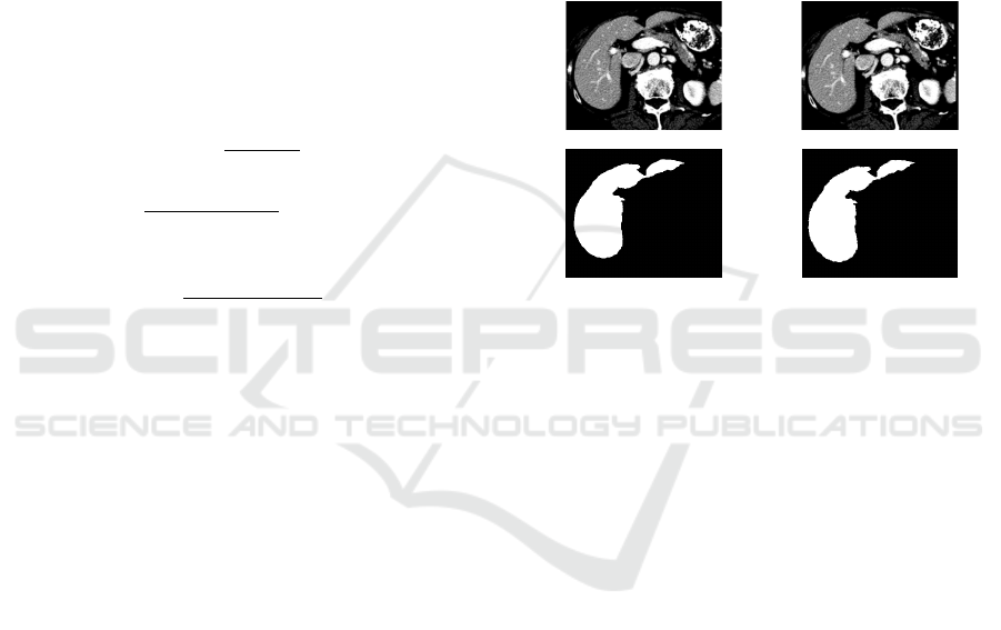
As shown in Fig. 2, all axial slices are scaled to the

target extent of 352×288 pixels with the intensity

profile of the target structure normalized around midst

position 127 of utilized data type unsigned char in

terms of data normalization, see Fig. 2 for slice 100 of

pre-processed dataset #0.

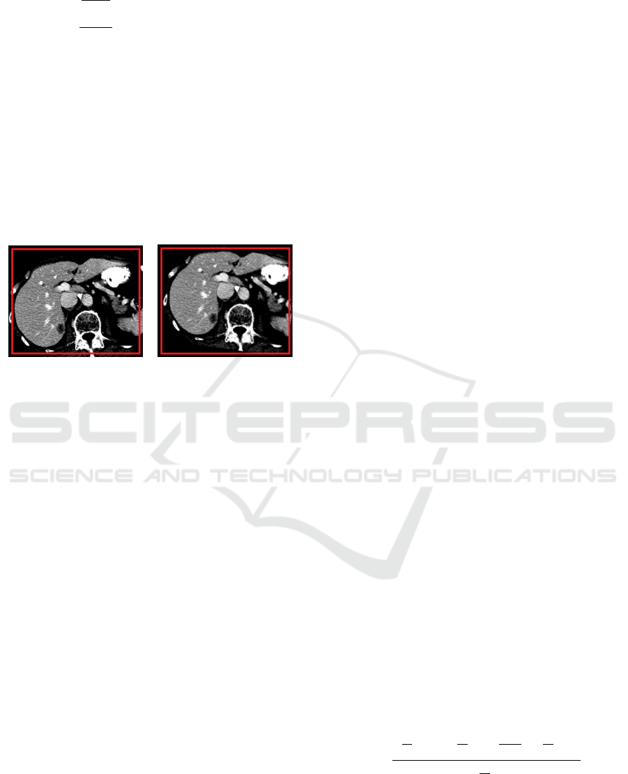
(a) (b)

Figure 2: The original slice 424 of dataset #0 (a) is cropped

according to reference segmentation mask with the average

pixel intensity of the liver parenchyma.

The given reference segmentations are of

acceptable accuracy and thus stay untouched with one

exceptional case, namely dataset #102 where around

slice 323 there is an invalid small blob classified

offshore the parenchyma that is removed.

3 METHODOLOGY

For liver segmentation based on tomographic 3D

volume data, several approaches for slice-wise

processing are evaluated and finally combined in a

hybrid model. For the segmentation task a U-net

VISAPP 2020 - 15th International Conference on Computer Vision Theory and Applications

architecture comprising 5 levels of hierarchy is

adjusted to input image size of 352×288 pixels for axial

slices, see Fig. 3. To prevent implicit shrinking by each

convolution operation, padding is applied, thus

ensuring intermediate image size reduced by a factor

of two at each hierarchy level, namely 176×144,

88×72, 44×36 and 22×18 respectively. The network

complexity is manifested by 31,031,685 trainable

parameters with kernel size 3×3 and considering the

bias parameters for each of the in total 23 layers.

3.1 Data Augmentation

With the liver dataset from the Medical Segmentation

Decathlon database only 131 tomographic CT volumes

are available. Nevertheless, as the volume is processed

in a slice-wise manner, the CT volumes result in at least

27,358 axial slices available for training, validation and

test. Due to the high resolution, differences between

neighbouring slices are low and thus redundancy is

present in the dataset. Thus, data augmentation is

needed to enrich the number of input slices to prevent

from over-fitting at higher epoch counts and to reduce

the gap between training and testing accuracy.

Data augmentation is implemented in an original

way to keep full control of the nature of the artificial

images generated compared to out of the box

Keras/Tensorflow functionality. The following

parameters are used to manipulate the slices chosen for

the current batch and thus to enrich the amount of data

available for training:

 transX and transY: translation in x-direction and y-

direction of the current slice

 rot: rotation around the image center

 intMul: linear scale of the image intensities leading

to brighter or darker pixel values within the borders

of the windowing range

 intAdd: additive manipulation of the intensities

within the window, leading to a uniform shift for

full scalar range

For all of these parameters, a valid range is configured

a priori. The parameter set to apply for a particular

image is then given as randomly selected values

(uniform distribution) within the valid range of the

augmentation parameters.

Pixel values of the augmented image are thereby

calculated as shown in Eqn. (2).





,











,





∙



1



0.5



∙







0.5



∙intAdd

(2)

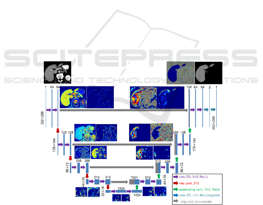
Figure 3: Network layout of the U-Net architecture utilized in this paper adapted from (Ronneberg et al. 2015). The intermediate

results on each of the five hierarchy layer are visualized for slice 72 of dataset #0. At full resolution of 352×288 two layers with

64 convolution kernels are applied while after reducing the size to 176×144 two layers with 128 convolution kernels each are

applied. To reconstruct the original size, four concat operators and up-sampling are applied.

Pre- and Post-processing Strategies for Generic Slice-wise Segmentation of Tomographic 3D Datasets Utilizing U-Net Deep Learning

Models Trained for Speciﬁc Diagnostic Domains





















∙

 

 







0.5



∙



0.5



∙



(3)

with  in



0.0;1.0



and 



0.5



∙.

A drawback of common data augmentation is the

loss of image information when rotating and

translating the image content while introducing

background regions with lack of information confusing

the model training process. To adress this problem and

to dampen the effects, a safety margin of

paddingOffset =10 is used to provide a

surrounding frame with original image data to use for

the augmented images, see Fig. 4.

(a) (b)

Figure 4: Although the axial slices utilized are of size

352×288, due to the paddingOffset the virtual image size is

372×308 thus introducing a safety margin for transformations

(a). With transX=15.5, transY=-23.8 and

rot=8.1 the relevant image content is still within the

processed as visible for the sinister rib cage (b).

3.2 Deep Learning based Classification

3.2.1 Classification of Axial Slices

In a straight-forward approach the tomographic input

datasets are sliced in axial direction to provide one-

channel input tensors of size 352×288 for the

modelAxial.h5 axial U-Net (ax) weights to be trained.

Due to the a priori defined ROI of the parenchyma area,

the axial parenchyma shape grows and shrinks in

caudal-to-cranial direction with moving position

according to a significant trend. Nevertheless, this

positional information within the slices is not utilized

in this approach.

According to the chosen pre-processing, the aspect

ratio of the axial slices is conserved with the width,

height scaled to the target tensor size utilizing cubic

interpolation. In z-direction there is no interpolation

required. All axial slices are varied with respect to data

augmentation parameters 16,16,10,.1,30 for

transX, transY, rot, intMul and intAdd respectively.

For model training, a learning rate of 5∙10



is configured for the Adam Optimizer (Kingma and Ba

2014) with 10.9 , 20.999 and

10



using cross-entropy as loss. The

training runs for 200 epochs at most using

32 and 12 preventing

from pre-mature stopping (validation loss).

3.2.2 Discrete Axial Model for Specific

Z-ranges within the ROI

With the model modelAxial.h5 neither 3D information

nor the characteristic axial liver shape according to the

position within the ROI are incorporated. Especially in

the caudal and cranial section of the ROI the

parenchyma size is low and varying intensity profiles

observed. Thus, the position within the ROI, denoted

as sliceRatio with values scaled to



0;1



should be

incorporated too.

For the chosen U-net architecture, it is hard to

provide the relevant sliceRatio parameter as additional

input to the network. It is possible to attach a FCN layer

with medium depth at the end of U-Net probability

mask classification to use the sliceRatio parameter for

automatic derivation of the locally best threshold value

for final binarization of the segmentation.

Nevertheless, there the positional impact would be

marginal.

As both the shape and position of the parenchyma

areas vary heavily within an entire 3D volume, splitting

the slice range into smaller sections increases the local

homogeneity at the cost of reduced amount of training

data, see Fig. 5.

To smooth transitions, the reduced amount of

training data for each of the sections as well as the

sharp border areas between them, the segments are

defined to overlap by 0.05 with [0;0.25[, [0.15;0.45[,

[0.35;0.65[, [0.55;0.85[ and [0.75;1.00] for the

sections 1-5 respectively.

To further utilize the predictability of neighbouring

segments close to the border sections, the final result is

combined in a linear interpolation way as shown in

Eqn. (4) with only the at most two sections

neighbouring the particular sliceRatio 



are

incorporated for number of classes 5 and model

predictions







,



∑



,

∙

,





with

(4)



,



















,





2∙

∙















VISAPP 2020 - 15th International Conference on Computer Vision Theory and Applications

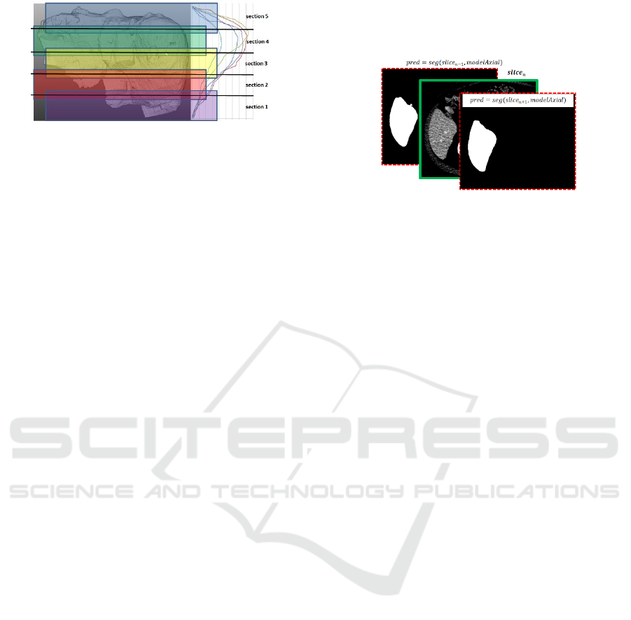
Figure 5: The axial slice stack is devided into overlapping

sections 1-5. As shown on the right chart, the position-related

trend in size for the first n=5 datasets is highly correlated and

thus motivates splitting into model sections.

3.2.3 Slice Propagation Incorporating

Neighbouring Results

Due to the high inter-slice-resolution of the employed

CT data, neighbouring slices show a high correlation

with respect to position, size and orientation of the

segmentations. Incorporating this given fact, the actual

slice segmentations are expected to get stabilized. A

similar semantic plausibility check is used with LSTM

deep learning for natural language processing or for

robust video object retrieval. Certainly, LSTM

concepts would be applicable too but enriching the

neighbouring slices with the right amount of

uncertainty at all memory layers is a challenging task.

Consequently, another 2D U-Net approach is

chosen and enriched with the neighbouring slices.

Besides the input 



to be segmented, also

autonomous segmentation results of the previous and

next slice as ,



and

,



are added to the input

tensor that is reshaped to



1,288,352,3



extent

similar as applicable for RGB images, c.f. Fig. 6.

A crucial aspect is how to define the neighbouring

slices for training. With the ground truth provided, the

influence of the particular intensity profile slice is

marginalized, thus only the proximate slices are

utilized.

The data augmentation for this 3-slice concept is of

high importance. The transformation of the mid slice is

performed with the same parameter set



16,16,10,.1,30



as used in section 3.1. To conserve

the inter-slice-correlation it would neither be a good

idea to randomly transform the proximate slices nor to

move them along with the mid slice to sustain a small

but crucial level of variability. Thus, for the previous

and next slice, a ¼ of the mid slice data augmentation

range is utilized and applied relative to the mid slice

transformation.

With the presented 3-slice model of

1,  and 

1 denoted as 



, the results of a first run can be

improved by bottom-up and top-down processing.

Furthermore, the slice-wise propagation opens rich

possibility for manual adjustment of the results.

Figure 6: The training tensor for the mid slice is enriched by

neighbouring single-slice predictions.

3.2.4 Incorporating Axial and Sagittal Views

for Overall Classification Building up a

Hybrid Position-based Model

The drawback of slice-wise data processing are the

outer sections, where the target structure continuously

vanishes in mass. For the axial slices, this is the case in

the top and bottom rows. To overcome this limitation,

it makes sense to incorporate sagittal and coronal slices

too. Although the sagittal and coronal slices show

weaknesses in the left/right and front/back areas

respectively, with respect to the overall information a

significant gain is expected. Axial slices are

transformed to sagittal (256x376) and coronal

(256x308) with z-dimension scaled to 256 for each of

the 3D datasets. Two U-net models, sagittal (ax

) and

coronal (ax

), are trained and applied as described in

section 3.2.1 with results back-transformed to axial

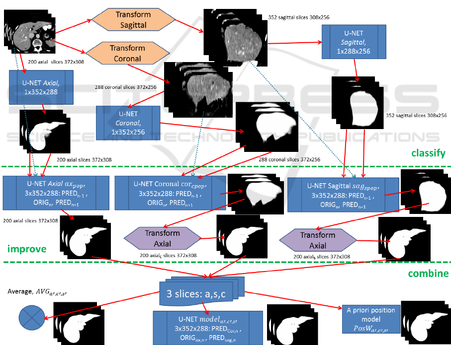
view. In Fig. 7 the preparation of segmentation results

for axial, sagittal and coronal can be seen in the

classify-section.

The 3-slice model ax

pop

, incorporating

neighbouring slices and thus a marginally perspective

aspect is expected to be capable of further improving

slice-by-slice results, c.f. improve section of Fig. 7.

With ax

pop

applied to reconstructions from sagittal and

coronal, axial segmentation information is thereby

already incorporated lowering the benefit for

combination of the three orthogonal views. Thus,

sagittal and coronal predictions are improved with

specific 3-slice models denoted as ax

spopSAG



and ax

spopCOR

respectively, see Fig. 7.

Now, as for each slice a good segmentation result

from axial, sagittal and coronal view is achieved, they

get combined for the final result.

The most straight forward approach thereby is

averaging of the three particular slices, denoted as





,,

. As for the border areas two of three views are

Pre- and Post-processing Strategies for Generic Slice-wise Segmentation of Tomographic 3D Datasets Utilizing U-Net Deep Learning

Models Trained for Speciﬁc Diagnostic Domains

expected to contribute good results, averaging or

majority voting seem to be a functional approach.

Alternatively, a 3-layer U-Net model can be trained

as decision tree, denoted as



,,

A third approach (



,,

) for combining the

orthogonal slices focuses on the position-based

evaluation of the prediction accuracy of the axial,

sagittal and coronal models calculated from pixel-wise

error as a normalized volume of size 100×100×100.

Smoothing (Gaussian kernel, r=1, 8 runs) is applied to

get a dense weight-map for position-dependent

accuracy of axial, coronal and sagittal slices.

4 IMPLEMENTATION

For the manually performed pre-processing steps such

as converting the image type, resampling to isotopic

voxels as well as for visualization of the results the

image processing frameworks and tools Analyze,

MeVisLab and ImageJ are utilized.

The model training and testing is implemented in

Python version 3.7.3 with separate parameterizable

scripts

for the various process steps using

Tensorflow 2.0 beta together with Keras.

The Python image processing is largely built upon

OpenCV or numpy for fast matrix operations.

To provide the model with training data, a

DataGenerator class is derived from Sequence

base class.

With a data generator, the batches can be loaded

from the file system on demand and one gets full

control on the data augmentation and on the batch-

randomization.

Figure 7: Axial slices are first transformed into sagittal and coronal views too, all to get classified by an individual U-Net. After

this classification section, results can further be improved by using a generic 3-slice U-Net (ax

pop

) after reconstruction to axial

view or specific ones (sag

pop

, cor

pop

) prior to axial reconstruction. The improved results finally get combined by one of the three

proposed strategies, averaging, U-net trained for merging or a position-based weighting algorithm.

VISAPP 2020 - 15th International Conference on Computer Vision Theory and Applications

5 RESULTS

5.1 Evaluation Metrics

For evaluation, in this work the same metrics as

proposed by the medical decathlon challenge are used

(MedDecathlon 2018). These are the Sørensen-Dice

coefficient (DSC)(Dice, 1945) for evaluation of the

spatial overlap and the normalized surface distance

(NSD) (Laplante, 2019) evaluating the spatial

proximity of test and reference shape to compare.

Additionally, the Jaccard index (Jaccard, 1912) as a

stricter metric for area match compared to the Dice

coefficient is evaluated too to allow for comparability

with further research papers. The metrics are calculated

according to Eqs. (5)-(7) for foreground reference

segmentation R and foreground test region S of image

I with ⊆,⊆ and pixels



,



∈∪.





,





2⋅

∩







(5)





,



1

∑





,



,



∙







,,

∑









,,

, 

,















(6)





,





∩









∩

(7)

Metric 



,



∈



0;1



thereby calculates for error

pixels the distance to the correct border of the reference

shape and normalizes with pixels in ∪.

For the overall accuracy of a dataset, i.e. 3D

volume, the metrics DSC, NSD and JI are caclulated

by summing up the FP, FN and correct results of all the

slices. To adress the statistics per slice, for the same

metrics a median slice accuracy is evaluated per dataset

denoted as DSC

med

, NSD

med

and JI

med

respectively.

Testing on several 3D volumes, the partciular results of

the six mentioned metrics are statistically analyzed too

for getting an overall evidence.

5.2 Hardware Infrastructure

All of the process steps discussed in this paper, namely

data preparation, pre-processing, model training and

validation/test are performed on a Colfax SX9600 GPU

Rack with 2×Intel Xeon Gold 6148 2.4GHZ processors

and 768GB of DDR4 memory with 2667MHZ clock

frequency split into 24 partitions of 32GB each. The

system runs CentosOS 7.6 operating system and

provides for fast tensor calculation 8 GPU cores,

namely 4× NVIDIA Volta Titan V 12G and 4× NVIDIA

Tesla V100 32G.

5.3 Results on Pre-processing and Data

Augmentation

The safety margin of 10 pixels used to enlarge the input

axial slices from 352×288 to 372×308 successfully

helped to prevent from black-areas due to rotation and

translation outside the image borders for the effective

image range. The intensity profile manipulation for the

data augmentation process does not result in a value

overflow, see Fig. 8.

To preserve the binary reference segmentation

masks, as interpolation strategy the modes Area and

Nearest Neighbour are to be utilized only.

(a)

(b)

(c)

(d)

Figure 8: Axial slice 276 (a) and reference segmentation (c)

get transformed by transX=-6.64, transY=3.51,

rot=3.00, intMul=1.02 and intAdd=-5.74 (b),

(d).

5.4 Slice-wise Classification Utilizing a

Single Model

The following axial, sagittal and coronal models are

trained with 22,000 (axial), 40,000 (sagittal) and

32,000 (coronal) augmented datasets while validation

is performed with the remaining datasets, namely

4,858 (axial), 8,232 (sagittal) and 7,848 (coronal). The

imbalance in train and test data results from different

dataset dimensionality in the main viewing directions

and is implicitly balanced utilizing data augmentation.

For results of the evaluation metrics on the axial,

sagittal and coronal model, c.f. Table 1. Furthermore,

the models ax

and ax

are evaluated after

reconstruction and resampling from sagittal/axial to

axial slices.

Although the axial, cornal and sagittal model show

similar accuracy, their particular strength is located in

various sections as shown in Fig. 9. The axial model is

weak in the caudal sections but outperforming in the

cranial sections.

Pre- and Post-processing Strategies for Generic Slice-wise Segmentation of Tomographic 3D Datasets Utilizing U-Net Deep Learning

Models Trained for Speciﬁc Diagnostic Domains

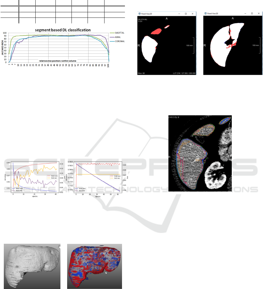
Table 1: Results for the particular slice-wise models

evaluated on the test datasets.

model DSC DSC

med

JI JI

med

NSD NSD

med



96.2 96.6 92.6 93.4 98.2 99.0





96.8 96.9 93.8 93.9 96.2 99.3





96.5 96.5 93.2 93.3 97.9 98.6

Figure 9: JI metric evaluated for axial, sagittal and coronal

model per 1% intervals with respect to relative z-position

within the volume.

The training process for the final axial model is

shown in Fig.10 (a) while in Fig.10 (b) an premature

stagnation with identical settings is visible. With each

epoch on full training data lasting for 35:10 minutes the

overall training of a large model took 15-20 hours. In

contrast, model evaluation takes place in millisecond

range and is only affected by file loading and pre-

processing demand.

(a) (b)

Figure 10: While in (a) the axial model approaches good

results within 36 epochs, depending on the initial random

batch and random the training gets early stuck in about 50%

of the cases (b).

(a)

(b)

Figure 11: Correctly segmented liver area for dataset #101 in

(a) and FP, FN visualization at surface and vena porta areas

in (b).

The achievable segmentation accuracy is

visualized for dataset #111 in Fig. 11 with the matching

volume in (a) and the FP and FN areas in blue and red

respectively. Axial segmentation results are rather

weak in the caudal and cranial areas, see Fig. 12. This

deficiency is easily levelled by incorporating sagittal

and coronal too, see Fig. 13.

(a) (b)

Figure 12: Axial view of segmentation mismatch of slice 88

and 135 of dataset #111 for model ax (a-b). In caudal

direction the starting slices of new morphological islands

sometimes stay unclassified.

Figure 13: Axial view of segmentation mismatch of slice 88

of dataset #111 with ground truth (green), axial (blue),

sagittal (red) and coronal (orange) incorporating the midst

parenchyma part (red FN region in Fig. 12 (a)) in caudal

direction in contrast to the axial result.

5.5 Classification with Discrete Axial

Models for Specific Z-ranges

Results on the section-based models are listed in Tab.

2. As the training data of 22.000 slices gets split up into

5 sections, the quality of these specific models are

marginally below the full axial model ax. Only if the

axial model is trained with a reduced amount of data

too for reason of compensation (axial small, ax

small

), the

section models are significantly outperforming. The

mode with linearly combining the classification results

of the neighbouring sections for a particular slice (e.g.

1,nb

) outperform the use of only the nearest section

(e.g. ax

VISAPP 2020 - 15th International Conference on Computer Vision Theory and Applications

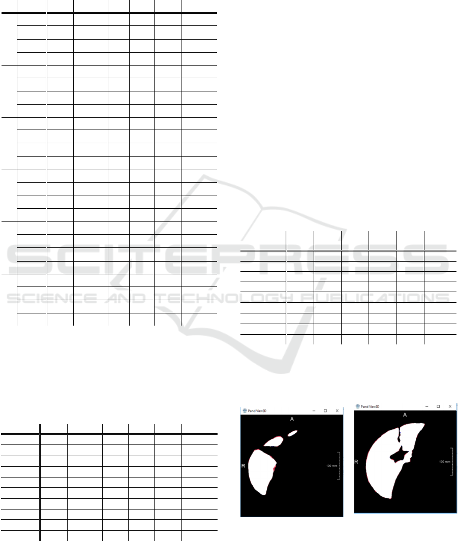
Table 2: Section based evaluation of various models,

namely full axial model ax trained with 22,000 datasets,

axsmall only trained with 4,400 datasets such as the section

models ax1- ax5. Model axnb incorporates neighbouring

sections for linear interpolation.

model

DSC DSC

med

JI JI

med

NSD NSD

med

ax 89.8 93.0 81.5 86.9 88.1 96.4

small

67.0 62.5 50.3 45.5 41.9 45.2

87.4 88.4 77.6 79.3 82.2 89.5

1,nb

88.0 89.3 78.5 80.6 83.6 90.9

ax 96.2 97.0 92.6 94.2 97.7 99.3

small

86.5 88.2 76.2 78.9 85.5 88.7

96.0 97.0 92.2 94.1 97.3 99.3

2,nb

96.2 97.2 92.6 94.5 97.6 99.4

ax 96.2 96.7 92.6 93.5 98.2 99.1

small

87.3 88.1 77.5 78.7 87.3 89.9

96.9 97.2 93.9 94.6 98.8 99.4

3,nb

96.9 97.1 93.9 94.4 98.8 99.4

ax 96.8 97.2 93.8 94.5 98.7 99.2

small

88.1 90.1 78.8 81.9 85.8 90.7

96.6 97.0 93.5 94.1 98.4 99.2

4,nb

96.9 97.2 94.0 94.6 98.7 99.4

ax 96.0 96.5 92.3 93.2 98.6 98.9

small

86.7 88.6 76.5 79.6 85.4 89.9

94.1 94.7 88.9 90.0 88.6 92.6

5,nb

94.6 95.1 89.7 90.7 90.2 94.5

all

ax 96.2 96.6 92.6 93.4 98.2 99.0

small

86.8 86.9 76.6 76.8 85.2 87.6

1-5

95.9 96.4 92.1 93.0 96.7 98.7

96.1 96.6 92.5 93.4 97.1 99.0

5.6 Slice to Slice Result Propagation

Results on the 3-slice U-Net implementing predictions

of the previous and the next slice are found in Table 3.

Table 3: Test runs on 3-slice model expecting prediction for

(n-1), original axial slice and prediction for (n+1).

model DSC DSC

med

JI JI

med

NSD NSD

med



96.2 96.6 92.6 93.4 98.2 99.0





95.2 95.6 90.8 91.5 95.1 98.6





97.0 97.3 94.1 94.7 98.7 99.4





98.6 98.5 97.2 97.0 99.9 99.9





96.8 96.9 93.8 93.9 96.2 99.3





97.2 97.3 94.5 94.7 98.0 99.2





97.1 97.1 94.4 94.4 97.2 99.1





96.5 96.5 93.2 93.3 97.9 98.6





96.9 97.1 94.0 94.4 98.3 99.1





96.9 97.0 93.9 94.1 98.2 99.0

The model is thereby trained to get the intensity

profile for slice n and a first rough prediction for the

slices n-1 and n+1. In Table 3 there are test runs for

three predictions as ax

ppp

, the expected input ax

pop

together with neighbouring predictions and ground

truth for previous (ax

top

). Furthermore, the

reconstructed sagittal and coronal slices are tested, too,

utilizing the same model. For the coronal and sagittal

view,

the axial 3-slice model (ax

spop

, ax

cpop

) leads to

similar improvements after reconstruction to axial

view as applying specific trained 3-slice models for

coronal and sagittal before the reconstruction (sag

spop

cor

cpop

), cf. Fig. 7.

5.7 Hybrid Position Model of Axial,

Coronal and Sagittal Segmentation

Combining the particular results from axial, coronal

and sagittal the overall quality of results gets improved

for the a priori position model and a U-Net trained for

combination.

Table 4: Quality of results for the segmentations ax, ax

and

is improved by combining with average (AVG), position

model (PosW) or U-net model trained for combination

(model). As input, the pre-classified slices without (a, s, c)

and with 3-slice improvement (a’, s’, c’) are applied.

model DSC

DSC

med

JI JI

med

NSD

med



96.2 96.6 92.6 93.4 98.2 99.0





96.8 96.9 93.8 93.9 96.2 99.3





96.5 96.5 93.2 93.3 97.9 98.6



,,

97.2 97.3 94.6 94.7 99.1 99.4



,,

97.2 97.3 94.6 94.7 99.1 99.4



,,

97.5 97.6 95.2 95.2 99.3 99.5



,,

97.4 97.5 94.9 95.1 99.2 99.5



,,

97.4 97.5 94.9 95.1 99.2 99.5



,,

97.6 97.7 95.3 95.5 99.4 99.6

Results on the entire liver dataset can be found in Table

4. Comparing the simple averaging (AVG) and the

complex position-based a priori model (PosW), the

results are almost equal.

(a) (b)

Figure 14: Axial view of segmentation mismatch of slice 88

and 135 of dataset #111 for model model

a’,c’,s’

(a-b). The 3-

slice model and combination of orthogonal views corrects the

error (model

a’,c’,s’

) of ax model, c.f. Fig. 12.

Pre- and Post-processing Strategies for Generic Slice-wise Segmentation of Tomographic 3D Datasets Utilizing U-Net Deep Learning

Models Trained for Speciﬁc Diagnostic Domains

It is shown that U-net models are applicable for result

migration too and highest accuracy is achieved for

utilizing both, the 3-slice-improvement and the

combination of the orthogonal views, c.f. Fig. 14 (a-b)

for slices 88 and 135 of dataset #111.

5.8 Comparison to Other Approaches

The highest achieved accuracy in this paper is to be

quantified with DSC=97.59, JI=95.29 and

NSD=99.37 for PosW

a’,c’,s’

A similar slice-based approach utilizing LevelSets

for result propagation and a Statistical Shape Model for

initial parametrization achieved an average

JI=93.6±3.3 and a volume match of 96.82±1.72%

(Zwettler et al. 2009). At the medical decathlon 2018,

the top team achieved DSC=0.95 and NSD=0.98

evaluated for L1 region utilizing a nnU-Net (Isensee et

al. 2019).

6 DISCUSSION

With precise pre-processing and post-processing, the

domain of 3D segmentation in medicine can be

addressed with 2D slice-by-slice models, too

approaching similar level of quality. Classification

with 2D models has some significant advantages with

respect to calculation power required for model

training and memory consumption. Furthermore, for

user-centric approaches in the medical domain, the

interaction with 2D slices is more common with a

broader range of interaction paradigms.

Surprisingly the sectional models did not pay of as

expected. It was shown that this fact results from the

reduced amount of testing data. Thus, if a sufficient

amount of slices is available, splitting into sectors is a

reasonable strategy, training only on a subset of the

axial shapes and positions besides the intensity profile.

With the data augmentation strategy presented in this

paper, the lack in training data could not be

compensated. Instead, real medical image data or

results of GANs should be utilized.

With the 3-slice model, the perfect basis for user-

centric and interactive post-processing is provided. In

this paper it was shown that the improved results can

be propagated from slice to slice. Nevertheless, the

axial

pop

model perfectly worked out for improving the

initially segmented slices at similar accuracy compared

to the particular models (sag

spop

, cor

cpop

). Marginal

incorporation of a mini 3D-subvolume of 3 slices

significantly improved results. In future incorporating

5 or 7 slices will be investigated, possibly a higher step

increment will allow further improvement.

The combination of the axial and reconstructed

coronal and sagittal results is a crucial point. As for all

positions two of the main views lead to robust results,

it is not a huge surprise that a simple averageing model

can compete with the presented complex a priori

position model. The concept, that axial is weak at

caudal and cranial directions with sagittal and coronal

weak at front/back and left/right respectively was

proven by deeper analysis.

Nevertheless, these aspects were not corrrectltly

adressed with the position-based model. The caudal

and cranial sections are not only axial slices at the very

begin or end as they might arise inside the volume too.

Thus, it would be a better strategy to analyze the local

gradients, e.g. utilizing eigenvalue analysis. If the x, y

or z-gradients are high in local neighborhood, one can

conclude the adapted weights for axial, coronal and

sagittal then.

With the chosen ROI size of 288×352×256 it was

shown that tensors for deep learning not necessarily

need to be isotropic as stated in other papers.

7 CONCLUSIONS

Utilizing powerful Deep Learning as a small image

processing module, most of its black box nature

vanishes. If these modules are integrated into

conventional image processing chains in an adequate

way, significant improvements on the date pre- and

post-processing become feasible.

Furthermore, it is shown that in spite of iteratively

improving deep learning architectures and processing

power it still might be a reasonable decision to

decompose a 3D segmentation problem into slice-by-

slice processing.

Future work will focus on user-centric interaction

paradigms. Up to now powerful deep learning models

are available for a broad community but rather as a

black box. Thus, one has to accept the most often good

results as they are provided by the model.

Nevertheless, in computer-based medical analytics

the human diagnostician always should have powerful

tools for overruling the machine made decisions. With

slice-wise processing of the input volume, many

human-computer interaction paradigms become

realizable.

Another aspect to address in ongoing research is the

genericity of this concept. Besides the parenchyma-

optimized ROI dimensionality all other aspects of the

model are very generic. With definition of a priori ROI

and windowing, one axial sagittal, coronal model

should be able to not only handle parenchyma data, but

also datasets with kidney, lung, gall bladder and many

VISAPP 2020 - 15th International Conference on Computer Vision Theory and Applications

more in focus too if getting re-trained on a sufficient

amount of reference data.

REFERENCES

Aggarwal, A., Vig, R., Bhadoria, S., and Dethe, C.G., 2011.

Role of Segmentation in Medical Imaging: A

Comparative Study. In: Int. Journal of Comp. Applic.

29(1).

Amorim, P.H.A., Chagas, V.S., Escudero, G.G., Oliveira,

D.D.C., Pereira, S.M., Santos, H.M., and Scussel, A.A.,

2017. 3D U-Nets for Brain Tumour Segmentation. In:

MICCAI 2017 BraTS Challenge. In: Proc. of the

MICCAI 2017.

Arik, S.O., Chrzanowski , M., Coates, A., Diamos , G.,

Gibiansky, A., Kang, Y., Li, X., Miller, J., Raiman, J.,

Sengupta, S., and Shoeybi , M., 2017. Deep voice: Real

time neural text to speech. In: ICML 2017

BIR, 1986. ANALYZE

Header File Format, available from

http://www.grahamwideman.com/gw/brain/analyze/for

matdoc.htm, last visted 11.9.2019.

Chen, C., Liu, X., Ding, M., Zheng, J., and Li, J., 2019. 3D

Dilated Multi-Fiber Network for Real-time Brain Tumor

Segmentation in MRI. In: CoRR, available from

https://arxiv.org/pdf/1904.03355.pdf, last visited

1.10.2019.

Christensen, A., and Wake, N., 2018. Wohler Report:

Medical image processing software, Available from

http://www.wohlersassociates.com/medical2018.pdf ,

last visited 1.10.2019 .

Cicek, Ö., Abdulkadir, A., Lienkamp, S.S., Brox, T., and

Ronneberg, O. 2016. 3D U-Net: Learning Dense

Volumetric Segmentation from Sparse Annotation. In:

MICCAI 2016.

Cootes, T.F., Taylor, C.J., Cooper, D.H., and Graham, J.,

1992. Training Models of Shape from Sets of Examples.

In Proc. of the British Machine Vision Conference, 9-18.,

Leeds, U.K.

Cootes, T.F., Edwards, G.J., and Taylor, C.J., 1998. Active

Appearance Models. In Proc. of the 5th Europ. Conf. on

Computer Vision, 484- 498. June 2-6, Freiburg,

Germany.

DFWG, 2005. NIFTI - Neuroimaging Informatics

Technology Initiative, available from

https://nifti.nimh.nih.gov/, last visited 11.9.2019

Dice, L.R., 1945. Measures of the Amount of Ecologic

Association Between Species. In: Ecology. 26 (3).

Frid-Adar, M., Diamant, I., Klang, E., Amitai, M.,

Goldberger, J., and Greenspan, H., 2018. GAN-based

synthetic medical image augmentation for increased

CNN performance in liver lesion classification. In:

Neurocomputing, pp. 321-331.

Goodfellow , I.J., Pouget Abadie , J., Mirza, M., Xu, B.,

Warde Farley, D., Ozair, S., Courville, A., and Bengio,

Y., 2014. Generative Adversarial Nets. In Proc. of the

27th Int. Conf. on Neural Information Processing

Systems, vol. 2.

Hochreiter, S., and Schmidhuber, J., 1997. Long Short-Term

Memory. In: Neural Computation 9(8), pp. 1735-1780.

Huang, C., Han, H., Yao, Q., Zhu, S., and Zhou, S.K., 2019.

3D U

-Net: A 3D Universal U-Net for Multi-Domain

Medical Image Segmentation. In: Proc. of the MICCAI

2019.

Isensee, F., Petersen, J., Kohl, S.A.A., Jäger, P.F., and Maier-

Hain, K.H., 2019. nnU-Net: Breaking the Spell on

Successful Medical Image Segmentation. In: CoRR.

Jaccard, P., 1912. The Distribution of the flora in the alpine

zone, In: New Phytologist, 11.

Kingma, D.P., and Ba, J.L., 2014. Adam : A method for

stochastic optimization. In: Int. Conf. on Learning

Representations (ICLR), available from

https://arxiv.org/abs/1412.6980, last visited 1.10.2019.

Laplante, P.A. (ed.), 2019. Encyclopedia of Image

Processing. In: CRC Press/Taylor & Francis Publishing.

McInerney, T., and Terzopoulos, D., 1996. Deformable

Models in Medical Image Analysis : A Survey. In

Medical Image Analysis 1 (2): pp. 91-108.

MedDecathlon, 2018. MSD-Ranking Scheme, available

from: http://medicaldecathlon.com/files/MSD-Ranking-

scheme.pdf, last visited 19.9.2019.

Meine, H., Chlebus, G., Ghafoorian, M., Endo, I., and

Schenk, A., 2018. Comparison of U-net-based

Convolutional Neural Networks for Liver Segmentation

in CT. In: Computer Vision and Pattern Recognition,

available from https://arxiv.org/abs/

1810.04017, last visited 1.10.2019.

Rajagopalan, S., Karwoski, R.A., Robb, R.A., Ellis, R.E., and

Peters, T.M., 2003. Shape-Based Interpolation of Porous

and Tortuous Binary Objects. In: MICCAI 2003, pp.

957-958.

Robb, R.A., Hanson, D.P., Karwoski, R.A., Larson, A.G.,

Workman, E.L. and Stacy, M.C., 1989. Analyze: a

comprehensive, operator-interactive software package

for multidimensional medical image display and

analysis. In: Comput Med Imaging Graph 13(6): 433–

454.

Ronneberg, O., Fischer, P., and Brox, T., 2015. U-Net:

Convolutional Networks for Biomedical Image

Segmentation. In: MICCAI 2015, Springer, LNCS,

Vol.9351: 234—241.

Simpson, A., Antonelli, M., Bakas, S., Bilello, M., Farahani,

K., Ginneken, B., Kopp-Schneider, A., Landman, B.,

Litjens, G., Menze, B., Ronneberger, O., Summers, R.,

Bilic, P., Christ, P., Do, R., Gollub, M., Golia-Pernicka,

J., Heckers, S., Jarnagin, W. and Cardoso, M.J., 2019. A

large annotated medical image dataset for the

development and evaluation of segmentation algorithms.

In CoRR.

Squelch, A., 2018. 3D printing and medical imaging. In:

Journal Med Radiat Sci. 65(3).

Stegmaier, J., 2017. New Methods to Improve Large-Scale

Microscopy Image Analysis with Prior Knowledge and

Uncertainty. In: KIT Scientific Publishing, Karlsruhe.

Strakos, P., Jaros, M., Karasek, T., Kozubek, T., Vavra, P.,

and Jonszta, T., 2015. Review of the Software Used for

3D Volumetric Reconstruction of the Liver. In: Int.

Journal of Computer and Information Engineering 9(2).

Pre- and Post-processing Strategies for Generic Slice-wise Segmentation of Tomographic 3D Datasets Utilizing U-Net Deep Learning

Models Trained for Speciﬁc Diagnostic Domains

Van Biesen, W., Sieben, G., Lameire, N., and Vanholder, R.,

1998. Application of Kohonen neural networks for the

non-morphological distinction between glomerular and

tubular renal disease. In: Nephrol Dial Transplant 13(1),

pp. 59-66

Viola, P., and Jones, M., 2001. Rapid Object Detection using

a Boosted Cascade of Simple Features. In: Conf. on

Computer Vision and Pattern Recognition 2001

Yang, D., Xu, D., Zhou, S.K., Georgescu, B., Chen, M.,

Grbic, S., Metaxas, D., and Comaniciu, D., 2017.

Automatic Liver Segmentation Using an Adversarial

Image-to-Image Network. In: MICCAI 2017.

Yi, X., Walia, E., and Babyn, P., 2019. Generative

Adversarial Network in Medical Imaging: A Review. In:

Medical Image Analysis vol. 58.

Zhang, J., and Wang, X.W. 2011. The application of feed

forward neural network for the X ray image fusion. In: J.

Phys.

Zwettler, G., and Backfrieder, W., 2013. Generic Model-

Based Application of Modular Image Processing Chains

for Medical 3D Data Analysis in Clinical Research and

Radiographer Training. In: Proc. of IWISH 2013, pp. 58-

Zwettler, G., Backfrieder, W., Swoboda, R., and Pfeifer, F.,

2009. Fast Fully-automated Model-driven Liver

Segmentation Utilizing Slicewise Applied Levelsets on

Large CT Data. In: Proc. of the 21

EMSS 2009, pp. 161-

166.

VISAPP 2020 - 15th International Conference on Computer Vision Theory and Applications