Decision Support for Shipping Spare Parts in Bundles

Yizi Zhou

, Jiyin Liu

, Rupal Mandania

, Kai Chen

and Rongjun Xu

Huawei Technologies Co Ltd, Bantian Huawei Base, Shenzhen, China

School of Business and Economics, Loughborough University, Loughborough, U.K.

Keywords: Parcel Delivery Pricing, Service Level Agreement, Optimisation, Mixed-Integer Programming.

Abstract: A telecommunication equipment company sends spare parts from local hubs to construction sites or other

local hubs in mainland China several times a day through parcel delivery services. Depending on the delivery

distance, there are various delivery options such as transportation via air, via road, via sea, via rail and via

inland waterways. Many choices named service levels are available within each transportation category. There

are three parcel delivery pricing policy: price per shipment, weight ranged price, and continuous pricing. Each

spare parts delivery usually has a priority level or delivery time requirement. Spare parts to be shipped from

the same hub or nearby hubs to the same or nearby destinations are considered being able to ship in bundles.

By observing the delivery pricing structure, it is usually beneficial to bundle spare parts together for shipment.

The problem is formulated as a mixed integer liner programming model. Numerical experiments are carried

out to observe the benefits and also reflect the features of parcel delivery pricing structure.

1 INTRODUCTION

We study a problem where a telecommunication

equipment company sends spare parts from local hubs

to construction sites or other local hubs in mainland

China twice a day. Typically, depending on the depot

hub and destinations of the shipment, there are

various means of freight transportation, such as

transportation via air, via road, via sea, via rail and

via inland waterways. Many choices named service

levels are available within each transportation

category. The service level agreement (SLA) is the

guaranteed delivery time of the parcel, e.g. the next

day by 18:00. The pricing of each delivery service is

different but typically increasing as SLA decreasing.

There are three types of parcel delivery pricing

policy. The first one is fixed price per shipment,

although there may be a limit on the maximum weight

or maximum number of items per shipment. This type

of delivery service is usually associated with truck

delivery or ship container delivery. The second

policy is range pricing with a minimum charge and a

unit price rate associated with each calculated

weight/volume range. Furthermore, the price can be

https://orcid.org/0000-0003-2140-801

https://orcid.org/0000-0002-2752-5398

https://orcid.org/0000-0002-9025-0569

of continuous charge with a fixed unit price and a base

charge. Express delivery services normally adopt this

kind of pricing policy. Calculated weight is the

maximum of the goods’ physical weight and the

volumetric weight. Volumetric or dimensional weight

is calculated based on the volume of the package

times the throw weight coefficient, and normally

international air transportation has a larger throw

weight coefficient than domestic road transportation.

One specific thing to take into consideration is the

price of shipping dangerous goods, such as liquid,

bio-hazardous substances. It requires additional

surcharges or charges at a higher unit price. Each

spare parts delivery usually has a priority level or

delivery time requirement. This requirement should

be met on or before SLA, the guaranteed delivery

time of the chosen delivery service. Spare parts

shipping from the same hub or nearby hubs to the

same or nearby destinations are considered to be able

to ship in bundles.

The traditional way is to send each spare part

separately once it is needed, or to bundle spare parts

with the same delivery time requirement. However,

this will incur more delivery cost and less profit

Zhou, Y., Liu, J., Mandania, R., Chen, K. and Xu, R.

Decision Support for Shipping Spare Parts in Bundles.

DOI: 10.5220/0008924803210328

In Proceedings of the 9th International Conference on Operations Research and Enterprise Systems (ICORES 2020), pages 321-328

ISBN: 978-989-758-396-4; ISSN: 2184-4372

321

margin. Moreover, this needs man hours on dealing

with each delivery order (e.g. tedious form filling

work). It will be beneficial to bundling spare parts

with different delivery time requirements together as

long as SLA satisfied all requirements for shipment.

For example, good A has a weight of 2kg and good B

has a weight of 1kg, both taking a range price delivery

option with 0-5kg, ￥1 per kg and minimum charge

of ￥5. Shipping these two goods separately will cost

￥10 and bundle them together only cost ￥5. This

simple example demonstrates the cost benefit of

shipment bundle. Given a set of spare parts to be

shipped, each with a delivery time requirement, from

one hub (or nearby hubs) to a destination hub (or

nearby hubs) and the available delivery options with

known pricing policies, the problem is to determine

how to bundle the spare parts to shipments so that the

total cost is minimised.

There has been research in the literature on

consolidation of shipments to save cost. For example,

Wong, et al (2009) and Li et al.(2012) studied the

shipment consolidation problems from the logistics

providers perspective. They formulate mixed integer

programming models to decide the consolidation of

shipments in different segments in the shipping

network to take advantage of economies of scale

while considering delivery target dates and handling

capacities. Nguyen et al. (2014) considered a problem

in which multiple suppliers consolidate their product

in long haul transportation to meet stochastic

demands of the perishable products. We have not

found previous research with the same settings as the

work in this paper which determines bundling of

shipments and selection of delivery services with

different pricing structures.

Section 2 of this paper demonstrates the features

of different delivery pricing policies. The above real-

life business problem can be abstracted and translated

using mathematical language. We formulate the

optimisation problem as a mixed integer linear

programming model with the objective of minimising

the total delivery cost. The decision variables are the

assignment of spare parts to delivery options which

reflects the bundles. The constraints are described

previously, including delivery time requirement and

the logistics of calculated delivery costs. The solution

approach and mathematical model is shown in section

3 and section 4. Numerical experiments are carried

out and explained in section 5. Section 6 gives some

real-life examples. Conclusions are drawn in section

2 DELIVERY SERVICE PRICING

There are many different ways of post service charges

and different regulations and strategies applied (Crew

and Kleindorfer, 2013; Marcus and Petropoulos,

2017; Wilson, 1993). Three main categories of postal

service pricing policy are explained in details, which

summaries the signed delivery service contracts in the

company. The first is price per shipment contract. It

computes cost by unit price per container times the

number of containers needed, and normally the

maximum capacity of a container is big enough for

half a day demand from the same locations.

The second type is range pricing for either weight

unit or volume unit. With the pricing unit in weight,

an example of this type of pricing policy is shown in

Table 1. This price policy applies to a certain route

and the transportation mode is by air. The guaranteed

delivery is within four days. For example, we have a

parcel to send with a weight of 21KG and a volume

of 0.003 ݉

ଷ

. Firstly, we need to compute the

calculated weight, which is the maximum of the

Table 1: Pricing policy of a supplier with weight range charges 4 days SLA.

Supplier SLA SHIP TYPE MIN CHARGE RANGE_FROM RANGE_TO UNIT RATE

A 4 BY AIR 400 0 5 KG 55

4 BY AIR 400 5 45 KG 42

4 BY AIR 400 45 300 KG 38

4 BY AIR 400 300 99999 KG 37

Table 2: Pricing policy of a supplier with continuous charges.

Supplier SLA SHIP

TYPE

MIN CHARGE

WEIGHT

MINI CHARGE ADJ RATE UNIT RATE

B 4 BY

EXPRESS

1 182 0.5 KG 45

ICORES 2020 - 9th International Conference on Operations Research and Enterprise Systems

322

goods’ physical weight and the volumetric weight.

Volumetric or dimensional weight is calculated based

on the volume of the package times the throw weight

coefficient, which is 167. The volumetric weight is

167 0.003 0.5, which is less than the weight so the

calculated weight is 21KG for this parcel. 21KG is in

the second range, so the unit price is 42. The

calculated price is 42 21 882 . This price is higher

than the minimum charge, so the final charge is 882

for this example. Similar calculation process applies

when the pricing unit is volume. The only difference

is when calculating the weight converted volume, we

use weight divided by the throw rate, which is a

different throw rate from previous 167. Furthermore,

the throw rate varies from country to country.

The third type of price policy is continuous charge

policy such as the one shown in Table 2. The formula

is quite different from that in the second one. The

calculated weight is equal to the maximum of the

goods’ physical weight and the volumetric weight. If

the calculated weight is not more than the minimum

charge weight, the price is the minimum charge.

Otherwise, the amount above the minimum charge

weight is rounded up to the nearest half and charged

based on the unit rate. For example, if a parcel has a

weight of 2.7KG and a volume of 0.05

ଷ

, using the

parameters in Table 2, the calculated weight is

max{2.7,0.05 167} 8.35

. The amount above the

minimum charge weight will be 8.35 1 7.35 KG

and rounded to 7.5KG. The charge for this part is

7.5 45 337.5 . Adding the basis charge, the final

charge for this parcel is then 519.5.

2.1 Features of the Pricing Policy

Structures

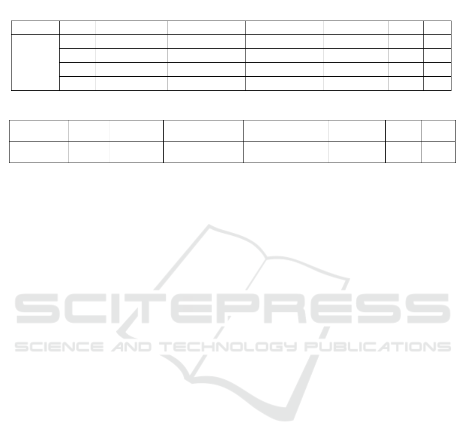
The weight range pricing policy has been plotted

partially for a parcel weight changing from 0KG to

50KG as shown in Figure 1. The bonus zone

[0, ]A

is where you can bundle as many as items into the

parcel and the total price would not change, where the

weight limit

/A MINI CHARGE RATE

Interestingly, the first price range does not take effect

as the calculated price will always be less or equal to

the minimum charges. In Figure 1, the arbitrage zone

[, ]BC

is where you can bundle more items or even

put package materials such as foam into the parcel to

reduce the total cost. The existence of an arbitrage

zone and a bonus zone verify the potential to reduce

total delivery cost by bundling items.

Figure 1: Partial plot of weight range pricing policy as in

Table 1.

The continuous pricing policy has been plotted

partially for a parcel weight changing from 0KG to

Table 3: Pricing policy of a supplier with weight range charges 3 days SLA.

Supplier SLA SHIP TYPE MIN CHARGE RANGE_FROM RANGE_TO UNIT RATE

A 3 BY AIR 400 0 5 KG 67

3 BY AIR 400 5 45 KG 52

3 BY AIR 400 45 300 KG 49

3 BY AIR 400 300 99999 KG 46

Table 4: Pricing policy of a supplier with weight range charges 2 days SLA.

Supplier SLA SHIP TYPE MIN CHARGE RANGE_FROM RANGE_TO UNIT RATE

A 2 BY AIR 600 0 5 KG 74

2 BY AIR 600 5 45 KG 68

2 BY AIR 600 45 300 KG 57

2 BY AIR 600 300 99999 KG 55

Decision Support for Shipping Spare Parts in Bundles

323

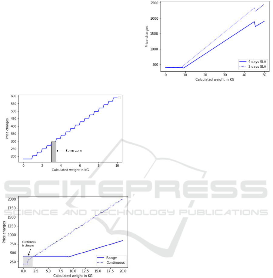
50KG as shown in Figure 2. It starts from a platform

according to the minimum charges and then moves

upwards as a staircase line. There are infinity many

small bonus zones like the one in Figure 1, but each

with a tiny width of 0.5KG. Those bonus zones are

created due to the round-to-half structure of the

pricing policy. The potential of reducing delivery cost

is much less than the range pricing policy. Figure 3

compares the pricing policy in Table 1 and Table 2.

When the weight of the parcel is less than or equal to

2KG, it is cheaper to choose continuous pricing

policy service; otherwise, it is better to send the parcel

with weight range pricing.

Figure 2: Partial plot of continuous pricing policy as in

Table 2.

Figure 3: Comparison of weight range pricing and

continuous pricing.

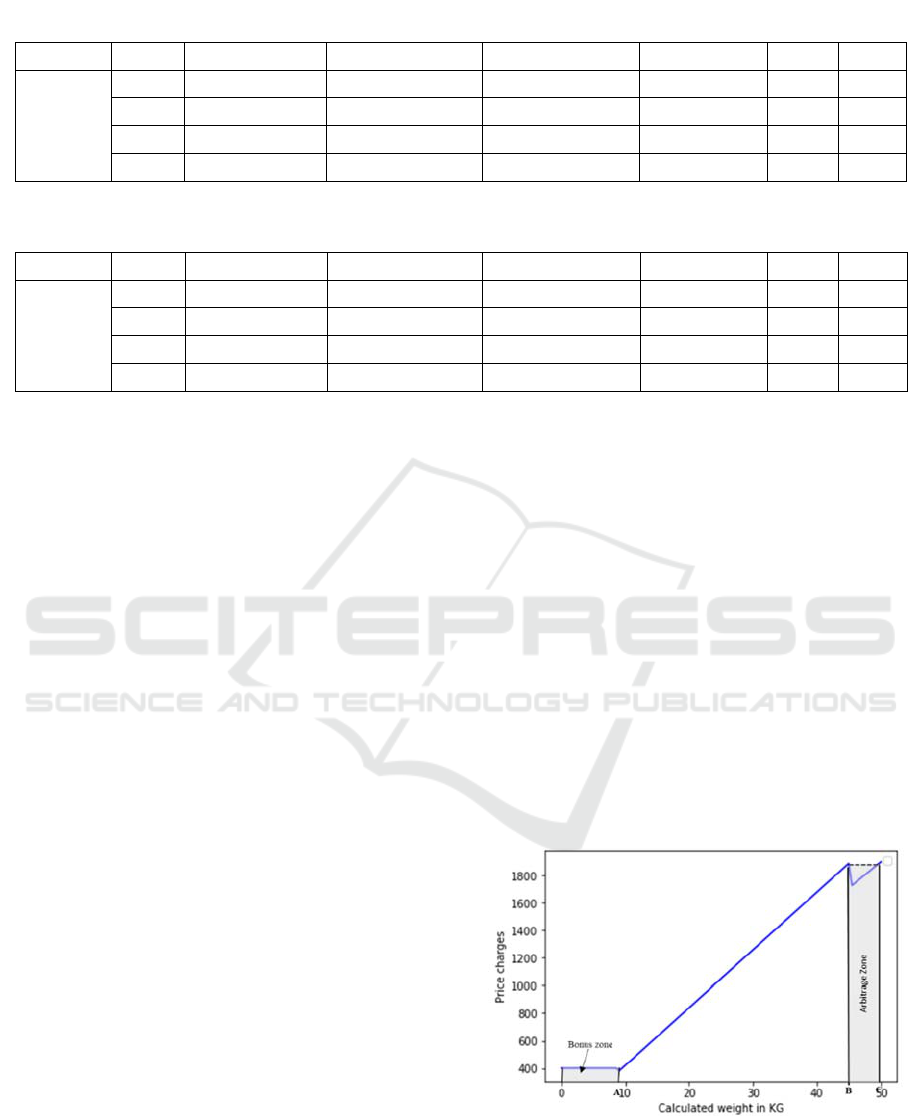
Figure 4 compares the same pricing policy structure

with different SLAs (weight range pricing). As the

data in Tables 3 and 4 show, the minimum charges of

3 days and 4 days are the same, but for every weight

range, 3 days service has a higher unit price rate. So

the service with 3 days SLA is in general more

expensive than that with 4 days SLA. In the situation

where the parcel is small and the price is the minimum

charge, a shorter SLA is more preferable. This should

be considered into the mathematical model as well.

With many different scenarios and combinations of

Figure 4: Comparison of weight range pricing with 4 days

SLA and 3 days SLA.

different SLA choices, it is extremely difficult to

solve the problem by hand or by searches guided by

rules found in this section, even given a long time. As

a consequence, we propose to formulate this problem

using mixed integer linear programming model. The

mathematical model can be solved by exact method

within seconds in most of the cases.

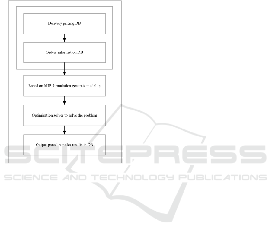
3 SOLUTION APPROACH

In the previous section, the features of different

delivery options with different SLA are

demonstrated.

The previous solution approach applied by the

company is to bundle orders by simple rules, which is

sending all orders with the same SLA in one parcel.

This is the rule based strategy for shipping spare parts

in bundles, but this may not lead to optimal solutions.

An alternative way to solve this is to formulate the

problem as a mathematically rigorous optimisation

problem, specifically a mixed integer programming

problem. The formulation is presented in section 4.

The solution framework is demonstrated in Figure 5.

4 MATHEMATICAL MODEL

A mixed integer programming model can be

formulated to demonstrate the problem of interest.

The objective is to minimise the total cost of all the

shipments after bundling spare parts. The constraints

are:



Orders from nearby depot hubs to nearby

destination hubs can be considered to be

bundled;



Delivery time requirement of each spare part

shipment must be satisfied;

ICORES 2020 - 9th International Conference on Operations Research and Enterprise Systems

324

 The pricing policy of each delivery option is

strictly followed;

 Dangerous goods are normally bundled with

dangerous goods and cannot be bundled with

ordinary goods.

Figure 5: Solution Framework.

4.1 Notations

Parameters:

i : index of spare parts that can be bundled together

: index of delivery options

: index of ranges in the range price policy

N : total number of spare parts

L : total number of ranges,

1, 3kKK

: set of indexes of all delivery options

: set of indexes of weight range price policy

delivery options

: set of indexes of continuous price policy

delivery options

: set of indexes of volume range price policy

delivery options

tr : delivery time requirement of spare part i

ts : service level agreement of delivery option

w : the weight of spare part i

v : the volume of spare part i

b : beginning weight/volume of price range

delivery option

, for 1, 3kKK

e : ending weight/volume of price range

delivery option

, for 1, 3kKK

u : unit price rate of range

of delivery option

, for

1, 3kKK



r : the throw weight coefficient of delivery option

for



d : the minimum charge of delivery option

, for



: the conversion rate of delivery option

, for



m : the minimum charge weight of delivery option

for

2kK

uc : unit price of delivery option

, for

2kK

: a big positive number.

Variables:



1,if spare part is allocated to delivery option

0, otherwise

X 



1, if the cost of delivery option is in range

0, otherwise







1, if at least one item is allocated to delivery option

0, otherwise





WL : bundle pricing calculated weight of delivery

option

1, 3kKK



, 0 if no spare part is

allocated to it

RWL : bundle pricing calculated weight of delivery

option

2kK

, 0 if no spare part is allocated

to it

C : total delivery cost of bundled spare parts of

delivery option k

4.2 Mixed Integer Programming Model

The mathematical model is formulated as follows

Minimise





(1)

Subject to:

1, [1,..., ]







(2)

, [1,..., ],

iik kik

tr X ts X i N k K  (3)

,1,2

kiik

WL w X k K K







(4)

,1,2

kkiik

WL r v X k K K







(5)

Decision Support for Shipping Spare Parts in Bundles

325

kik

WL X k K







(6)

kiik

WL v X k K







(7)

ik k

MkK









(8)

kik









(9)

,1,3

lk k

kKK









(10)



(1 ) (1 ) ,

1, 3, 1,...,

lk lk k lk lk

bMWLeM

kKKl L



   

 

(11)





(1 ) , 1, 3, 1,...,L

klkk lk k

CuWL MkKKl



 

(12)

(1 ) ,

kk k

Cd M kK



  (13)



(1 ) , 2

kk k k

RWL m

Cd uc M kK





  

(14)

2 2 0.99999, 2

kkk

WL RWL WL k K 

(15)



, {0,1}, , 1,...,

ik k

kKi N





(16)



{0,1}, 1, 3, 1,...,

lk k

kKKl L



 

(17)

,0,

WL C k K (18)

is integer

RWL (19)

The objective (1) of the model is to minimise the

sum of delivery cost of all delivery options, and if

there is no spare parts allocated to a certain option,

C  . Once there is a tie on price we will choose

the fastest delivery option in the post processing

check. Constraints (2) indicate that a spare part must

be allocated to exactly one delivery option.

Constraints (3) ensure that if spare part

i is allocated

to delivery option

, then the required time of spare

part

i (e.g. 3-day arrival) must not be shorter than the

guaranteed delivery time of option

(e.g. 2-day

SLA). In the program, we modelled constraints (3)

such that if

, [1,..., ],

tr ts i N k K , then

X 

. Constraints (4) and (5) compute the sum of

calculated weight of delivery option

1, 2kKK ,

which is sum of the maximum weight (max of

physical weight or volumetric weight) of all spare

parts allocated to it. Constraints (6) and (7) compute

the sum of calculated volume of delivery option

3kK

, which is sum of the maximum volume (max

of physical volume or weight converted volume) of

all spare parts allocated to it. Constraints (8) and (9)

define that





means at least one spare part is

allocated to delivery option

. Then constraints (10)

require that if delivery option

is used, the

calculated weight/volume of spare parts to be

delivered using option

must fall into one and only

one range. Constraints (11) identify the right range

[,]

lk lk

be of delivery option 1, 3kKK which the

calculated weight falls in. Constraints (12) and (13)

calculate the total cost of delivery option

1, 3kKK

which is the maximum of the minimum charge and

the unit price times the calculated weight/volume.

Constraints (13), (14) and (15) calculate the total cost

of delivery option

2kK



which is the maximum of

the minimum charge and the continuous price charge

as stated in section 2. Constraints (15) ceil the

calculated weight

WL to the nearest half. One may

notice that

WL is defined for 1, 3kKK as well,

but calculated differently in constraints (15) for

2,kK



as for continuous price the calculated

weight is rounded every 0.5kg. In a word,

,WL WL

can be viewed as a different variable as

WL . The rest

constraints state that all decision variables are greater

or equal to zero, among them

ik k lk





are binary

variables and

RWL only take integer values. For

dangerous goods, a separate problem will be

considered and solved using the same model, as they

cannot be shipped together with other spare parts.

5 NUMERICAL EXAMPLES

Three numerical examples are generated and selected

from real life data. The mathematical models are

solved using open source optimiser COIN-OR’s

COIN Branch and Cut Solver (CBC) under the

Eclipse Public License (Forrest and Lougee-Heimer,

2005). All test cases are run on a 2.11GHz Intel Core

i7-8650U (8 cores, 16GB) laptop.

5.1 Example One

The first example from real life data is shown in Table

5. The suppliers and price list are shown in Tables 1-

4. Among the five different options (suppliers and

price policies), the first three are selected. It is

ICORES 2020 - 9th International Conference on Operations Research and Enterprise Systems

326

interesting that item 2, 3, 4 required 4 days to arrive

are allocated to delivery option three with 3 days SLA,

and by doing this is the minimum-cost delivery plan.

The minimum total cost of sending these six items are

2292.21 with a computational time of 0.23 seconds.

If the items are sent out separately each in one parcel,

the total cost are 2593 (11.6%). If the items are

bundled by the same SLA, for example, items 2, 3, 4

can be bundled together and sent with 4 days service,

the total cost are 2367.45 (3.18%). The percentage of

the reduction in delivery cost of our plan is shown in

bracket.

Table 5: Example one item details.

INDEX SLA WEIGHT VOLUME Bundle

1 3 3.8 0.05 2

2 4 2 0.05 3

3 4 2.2 0.05 1

4 4 14.2 0.14 3

5 2 9.5 0.07 1

6 3 10.25 0.06 2

5.2 Example Two

This example demonstrates the importance of the

second objective functions, once there is a tie on the

delivery cost of different options. As all the items

require the same SLA, it is obvious to bundle all items

and send them with the four days SLA delivery

options. The delivery cost of the bundle with four

days delivery option is 400. However, the delivery

cost of the bundle to be shipped with three days SLA

is also 400, as demonstrated in Figure 4, the bundle

weight is in the bonus zone. With the second

objective function, when optimizing for this objective,

we only consider solutions that would not degrade the

objective values of delivery cost objectives.

Table 6: Example two item details.

INDEX SLA WEIGHT VOLUME Bundle

1 4 1 0.001 1

2 4 1 0.001 1

3 4 1 0.001 1

4 4 1 0.001 1

5.3 Example Three

This example shows an interesting case, where we

can add packing material into the parcel to increase

its weight and get a cheaper deal. The calculated

weight of the bundle is 44kg, corresponding to the

delivery option in Table 1. The delivery cost of the

bundle with 44kg is 1848, while we could add a little

bit weight to the current bundle and push it to the

arbitrage zone as shown in Figure 1. The optimal cost

of the bundle shipment is just above 1710, while we

augmented the parcel weight to just above 45kg. This

optimal cost is also found by solving the MIP problem.

Table 7: Example three item details.

INDEX SLA WEIGHT VOLUME Bundle

1 4 20 0.001 1

2 4 10 0.001 1

3 4 10 0.001 1

4 4 4 0.001 1

6 NUMERICAL EXPERIMENTS

The program is applied into one department’s daily

business since earlier this year and achieved around

17% savings on delivery cost every month comparing

to the same time period of last year. The program is

run several times daily and we selected 20 examples

from real life business to demonstrate the benefits of

applying this program. One example is one batch of a

particular day. The ORDERS column is the total

number of orders to be dispatched at that time period

of that day, and OPT_GROUPS column is the optimal

parcel numbers after we bundled shipment. The ratio

column is the bundle ratio, which is calculated as the

number of groups divided by the number of original

orders. The TIME column is the computational time

of the optimization problem.

In Table 8, we selected 20 batches of orders to be

dispatched. The average bundle ratio for this example

by the proposed optimisation program is 0.387. The

average computational time is 1.58 minutes. The

comparison between the new solution approach and

the traditional solution approach is shown in Table 9.

We increased the bundle ratio by 53.6%, which

means we largely reduced the packing time and

efforts for parcels. More importantly, the unit price

for sending those parcels before optimisation is 8.5

and after optimisation is 7, which indicates a 17.49%

reduction in delivery cost.

7 CONCLUSIONS

A telecommunication equipment company sends

spare parts from local hubs to construction sites or

other local hubs in mainland China several times a

day through parcel delivery services. Depending on

the delivery distance, there are various delivery

options such as transportation via air, via road, via

Decision Support for Shipping Spare Parts in Bundles

327

sea, via rail and via inland waterways. Many choices

named service levels are available within each

transportation category. There are three parcel

delivery pricing policies: price per shipment, weight

ranged price, and continuous pricing. Each spare parts

delivery usually has a priority level or delivery time

requirement. Spare parts to be shipped from the same

hub or nearby hubs to the same or nearby destinations

are considered to be able to ship in bundles. By

observing the delivery pricing structures, it is

beneficial to bundle spare parts together for shipment.

The company used to bundle shipment by hand,

following the rules of sending orders with the same

delivery time requirement in one parcel. We proposed

a new solution approach to tackle this problem. A

mixed integer programming problem is proposed

based on the delivery requirements as well as the

various ways to compute delivery cost based on

different delivery modes. Numerical experiments

have been carried out to observe the benefits and also

reflect the features of parcel delivery pricing

structures. Then 20 real life business examples are

selected. The average computational time is 1.58

minutes. Comparing to the traditional solution

approach, we are able to increase the bundle ratio or

in other words reduce the total number of parcels sent

by 53.6% while keeping the same number of orders.

This means that the time and efforts spent packing

parcels are greatly reduced. Furthermore, the total

delivery cost is reduced by 17% by using the new

solution approach.

Table 8: Real life examples.

ORDE

OPT

GROU

Ratio TIME

1 210 100 0.476 0.933

2 790 235 0.297 2.383

3 145 36 0.248 0.367

4 161 69 0.429 0.667

5 158 75 0.475 0.717

6 307 121 0.394 1.267

7 640 219 0.342 2.250

8 94 39 0.415 0.400

9 145 51 0.352 0.500

10 136 69 0.507 0.650

11 147 56 0.381 3.550

12 267 132 0.494 1.250

13 104 50 0.481 0.500

14 941 247 0.262 6.050

15 353 146 0.414 1.250

16 963 257 0.267 3.017

17 206 80 0.388 0.767

18 737 257 0.349 2.600

19 208 83 0.399 0.817

20 459 171 0.373 1.700

0.387 1.582

Table 9: Comparison with previous solutions by hand.

ders Groups Ratio Unit

Cos

By han

7171 5378 0.75 8.5

rogra

7171 2493 0.387 7

REFERENCES

Crew, M.A., Kleindorfer, P.R. eds., 2013. Postal and

delivery services: pricing, productivity, regulation and

strategy. Springer Science & Business Media.

Forrest, J., Lougee-Heimer, R., 2005. CBC user guide. In

Emerging theory, methods and applications. pp. 257-

277. INFORMS.

Li, Z., James H.Bookbinder, J.H. and Elhedhli, S., 2012,

Optimal shipment decisions for an airfreight forwarder:

Formulation and solution methods, Transportation

Research Part C: Emerging Technologies, 21(1),

pp.17-30.

Marcus, J.S., Petropoulos, G., 2017. E-commerce in

Europe: Parcel delivery prices in a digital single market.

In M. Crew, P. L. Parcu and T. Brennan (edd) The

Changing Postal and Delivery Sector, pp. 139-159.

Springer, Cham.

Nguyen, C., Dessouky, M. and Toriello, A., 2014,

Consolidation strategies for the delivery of perishable

products, Transportation Research Part E: Logistics

and Transportation Review, 69, pp.108-121.

Wilson, R.B., 1993. Nonlinear pricing, Oxford University

Press.

Wong, W.H., Leung, L.,C. and Hui, Y.V., 2009, Airfreight

forwarder shipment planning: A mixed 0–1 model and

managerial issues in the integration and consolidation

of shipments, European Journal of Operational

Research, 193(1), pp.86-97.

ICORES 2020 - 9th International Conference on Operations Research and Enterprise Systems

328