Hierarchical Traffic Sign Recognition for Autonomous Driving
Vartika Sengar
1
, Renu M. Rameshan
1
and Senthil Ponkumar
2
1
School of Computing and Engineering, Indian Institute of Technology, Mandi, Himachal Pradesh, India
2
Continental Automotive Components Pvt. Ltd., Bengaluru, Karnataka, India
Keywords:
Hierarchical Classification, Spectral Clustering, Convolutional Neural Networks, Machine Learning, Data
Processing, Image Processing, Pattern Recognition.
Abstract:
Traffic Sign Recognition is very crucial for self-driving cars and Advanced Driver Assistance Systems. As
the vehicle moves within a region or across regions, it encounters a variety of signs which needs to be recog-
nized with very high accuracy. It is generally observed that traffic signs have large intra-class variability and
small inter-class variability. This makes visual distinguishability between distinct classes extremely irregu-
lar. In this paper we propose a hierarchical classifier in which the number of coarse classes is automatically
determined. This gives the advantage of dedicated classifiers trained for classes which are more difficult to
distinguish. This is an application oriented work which involves systematic and intelligent combination of
machine learning and computer vision based algorithms with required modifications for designing fully auto-
mated hierarchical classification framework for traffic sign recognition. The proposed solution is a real-time
scalable machine learning based approach which can efficiently take care of wide intra-class variations with-
out extracting desired handcrafted features beforehand. It eliminates the need for manually observing and
grouping relevant features, thereby reducing human time and efforts. The classifier performance accuracy
is surpassing the accuracy achieved by humans on publicly available GTSRB traffic sign dataset with lesser
parameters than the existing solutions.
1 INTRODUCTION
In recent times there is a rapid growth in the field of
intelligent transport system and self driving cars. The
revolution in the field of autonomous cars is accom-
panied by the growth in the field of advanced driv-
ing assistance systems which redefines the quality of
driving experience and safety (Thrun, 2010). Traf-
fic sign recognition (TSR) systems are used to as-
sist the driver, and to direct the AI systems of au-
tonomous cars. TSR is a challenging task as it has to
deal with traffic signs belonging to different countries
having different number of traffic sign categories. The
real-time automated TSR system should have a high
recognition rate and less execution time. It comprises
of broadly three levels: Region of interest (ROI) pro-
posal, ROI classification and tracking. This work fo-
cuses mostly on the classification part.
In sign classification, some traffic sign classes
are harder to distinguish than others. Such difficult
classes need exclusively designed classifiers. Keen
observation is required in grouping different sign
classes to have better recognition. Manual grouping
of the different category of signs and its analysis is
time prone and sometimes error prone too. Automat-
ing the classification of sign classes guided by ma-
chine learning is essential. This automation can be
efficiently handled by a hierarchical classifier which
is capable enough to make the effortless inclusion of
the new category of signboards.
To build a hierarchical classifier, using a bank of
classifiers (e.g.: SVM, Adaboost, Polynomial Classi-
fier etc.) is still a widespread method in the current
industry. These classifiers are trained by manually
grouping similar kind of sign features together and
are combined properly in a hierarchy to automate the
grouping of different sign classes (Wang et al., 2013).
Seeing the hierarchical classifier as a decision tree,
the root classifier can be trained to distinguish among
the shapes of traffic signs like triangular, rectangular
and circular. Following the root node, more dedicated
classifiers can be trained which can classify amongst
the circular signs, say, using background and rim col-
ors. At the root node of the tree, all classes are avail-
able for classification. As we go down the category
tree, the number of categories for classification de-
308
Sengar, V., Rameshan, R. and Ponkumar, S.
Hierarchical Traffic Sign Recognition for Autonomous Driving.
DOI: 10.5220/0008924703080320
In Proceedings of the 9th International Conference on Pattern Recognition Applications and Methods (ICPRAM 2020), pages 308-320
ISBN: 978-989-758-397-1; ISSN: 2184-4313
Copyright
c
 2022 by SCITEPRESS – Science and Technology Publications, Lda. All rights reserved

creases.
The existing hierarchical classifier has some draw-
backs. Firstly, classifier at each node works as a flat
classifier focusing only on those classes for which the
particular classifier was trained. It does not consider
the relationship between other nodes. Secondly, it is
complex to train the classifier and lesser performance
in the upper level leads to even lesser performance
in the lower levels. The third disadvantage is the
need for manually observing and grouping relevant
features which needs human time and effort. This
calls for a solution which does not require handcrafted
features and manual grouping. Convolution neural
network (CNN) (LeCun et al., 1999) are known for
learning features relevant to the problem. Using weak
CNN based classifier we learn the category hierar-
chy. This eliminates the need for human in the loop
thereby reducing human efforts. Another major ad-
vantage of using CNN is scalability and less complex
design in terms of parameters and architecture. The
model should easily adapt to the class level changes
and database changes. The work done is not restricted
to sign recognition problems and has the flexibility to
address any type of classification challenges, example
visual object classification.
We propose a simple modification which leads to
gain in performance. The main contributions of this
work are:
• We use the hierarchical CNN for image classifica-
tion (Yan et al., 2015) with modifications for TSR.
In (Yan et al., 2015) the number of fine classifiers
which are dedicatedly trained for similar classes,
are fixed apriori. This is not suitable for our appli-
cation. So, we adopted a method for automatically
determining the number of fine classifiers. This is
one of the major contribution of our work.
• The second contribution is extensive analysis of
performance of hierarchical classifier leading to
several methods of improving the performance
and achieving a performance better than human
for publicly available GTSRB dataset. The archi-
tecture is evaluated and analyzed in detail for both
publicly available GTSRB dataset and Triangular
sign dataset collected in-house.
The paper is organized as follows. Sect. 2 describes
review of related literature. Sect. 3 explains the archi-
tecture and method for designing hierarchical classi-
fier framework. The experimentation details and re-
sults is presented in Sec. 4. The analysis of experi-
mentation done is described is Sec. 5. Finally, con-
clusions and future work is discussed in Sec. 6.
2 LITERATURE SURVEY
The idea of learning category hierarchies and using
it for image classification problem has been there
since a very long time. The initial works by (Gavrila,
1998), describes a multi-feature hierarchical method
to match N objects of different classes with a test im-
age using distance transforms. The novelty in this
idea was that N templates are grouped offline based
on similarity and form a template hierarchy. Similar
templates were grouped and represented by a proto-
type template. At every intermediate level of hier-
archy, matching is done using these prototype tem-
plates and at the leaf level all N templates are avail-
able for matching. In the last ten years, deep learning
solutions have become prevalent for hierarchical clas-
sification problem. (Zhu and Bain, 2017) suggested
branch convolution neural network for hierarchical
classification. In (Zhu and Bain, 2017) a CNN model
was proposed which contains several branch networks
along with a main convolution branch. The output of
the model are multiple predictions from coarse to fine
level but the category hierarchy should be known in
advance. (Xiao et al., 2014) explains an incremen-
tal learning approach in CNN. As new classes arrive
training algorithm grows a network either incremen-
tally or hierarchically according to the similarities be-
tween the classes. The model inherits feature from an
existing Alexnet architecture. (Xuehong Mao et al.,
2016) uses hierarchical classification particularly in
the domain of traffic sign recognition. Here, the mea-
sure of similarity between the categories is calculated
by transferring the images in the frequency domain
and then calculating Hadamard matrix product to get
a similarity metric. Here the similarity metric is gen-
erated by processing training data. A CNN oriented
family clustering is done based on similarity metric
to obtain the category hierarchy. In the work dis-
cussed in this paper, no processing is done on training
data to obtain the similarity metric which is used for
learning category hierarchy. The network itself learns
the category hierarchy from the confusion matrix of a
pre-trained model. In (Yan et al., 2015) category hi-
erarchy is learned automatically using spectral clus-
tering of confusion matrix by grouping those classes
which can easily be confused. The number of groups
formed are predefined in (Yan et al., 2015). In (San-
guinetti et al., 2005) an algorithm for pre-determining
the groups in spectral clustering is proposed. We have
used this algorithm to automatically identify the op-
timal number of groups required. Followed by this,
dedicated networks for these groups can be trained
parallelly for classification by using weighted predic-
tion averaging. The work is explained in more details
in next sections.
Hierarchical Traffic Sign Recognition for Autonomous Driving
309

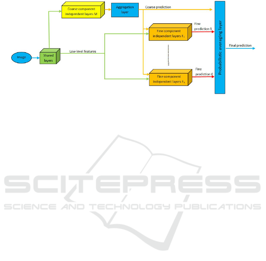
Figure 1: Hierarchical Convolutional Neural Network Architecture.
3 THE PROPOSED APPROACH
Hierarchical classifier design for traffic sign recogni-
tion is implemented by combining CNNs in the two-
level category hierarchy (Yan et al., 2015). The CNN
at the root level known as coarse category classifier
is used to classify those classes which can be easily
distinguished. At the second level, fine classifiers are
trained for each coarse category. Each fine classifier is
used to distinguish between the classes which are dif-
ficult to discriminate. Thus, these dedicated fine clas-
sifiers are expected to improve the classification accu-
racy. The architecture and algorithm are discussed in
further subsections.
3.1 Architecture and Algorithm
The network architecture mainly comprises of four
components as shown in Fig. 1. The details of these
components are given in Table 1. The building block
can be any CNN architecture which performs well as
a classifier on the given dataset. The building block
layers, its configuration and output size are shown in
Table 2. The architecture used is similar to VGG ar-
chitecture as it uses 3 × 3 convolution filters and
number of filters increases as we go deeper into the
network. The shape of the input RGB image is taken
as 64 × 64 × 3. The concept of shared layers is
useful because of the fact that low-level features are
important for both coarse and fine classification. So,
lower layers of CNN can be shared which leads to
lesser computations, parameters and memory require-
ments. The overall algorithm for the two-stage hier-
archical classification is detailed in Algorithm 1.
3.2 Learning of Category Hierarchy
Spectral clustering is used to learn the category hier-
archy automatically i.e., to group similar fine classes
together to form a coarse category and for each such
coarse category, k, an exclusive fine category classi-
fier, F
k
, is trained. This is obtained by doing spec-
tral clustering on a confusion matrix F ∈ R
CXC
ob-
tained from flat classifier which is trained to classify
all C fine categories. Note that a bad classifier leads
to a better clustering. For complex clustering prob-
lems where data cannot be separated by a hyperplane
eg., concentric circles, spectral clustering algorithm
(Ng et al., 2002) is used by transforming original data
into a new transformed space in fewer dimensions us-
ing Laplacian eigenmaps (Vidal, 2011). In ideal case,
when data-points of K different groups are not con-
nected and the connections are present only within the
group then Laplacian matrix will have exactly K num-
ber of zero eigenvalues. After embedding to a space
of fewer dimension, all N data-points map exactly to
K distinct points. The spectral clustering algorithm
is explained in (Ng et al., 2002). In original spectral
clustering algorithm value of K should be known in
advance. In next subsection, algorithm is discussed
for determining the value of K automatically.
3.3 Algorithm for Determination of
Optimal Number of Clusters
If instead of selecting first K eigenvectors, q eigen-
vectors are selected where q < K this means that q-
dimensional subspace in clustering space is selected.
Earlier, the transformed points cluster around K mutu-
ally orthogonal vectors, now their projection in lower
dimensional space will cluster along radial directions.
So, clusters will be elongated in the radial direction.
ICPRAM 2020 - 9th International Conference on Pattern Recognition Applications and Methods
310

Table 1: Architecture Description.
Component Layer Configuration
Shared layers Take input as image and extract low-level features. These are
preceding layers from building block CNN.
Single Coarse Category Classifier, M Generate intermediate fine predictions,
n
M
f
i j
o
C
j=1
, for image
x
i
with label y
i
. It comprises of end layers from building block
CNN. Here C is the total number of fine categories.
Fine-to-coarse aggregation layer Generate a coarse class prediction, M
ik
for coarse category k
and image x
i
, from intermediate fine predictions using many
to one mapping, P : [1,C] 7→ [1, K], where K is the number
of coarse categories formed after grouping fine categories.
Coarse class predictions are used as weights to combine fine
classifier predictions.
K Fine category Classifiers,
{
F
k
}
K
k=1
Generate fine prediction, P
k
(y
i
= j | x
i
) by fine component
F
k
, over a partial group of classes for which it is dedicatedly
trained for and probabilities of other fine classes which are not
present in the group are set to zero. Layer configuration is the
same as building block CNN but the number of neurons in the
final output layer is equal to the number of classes present in
the partial set instead of the total number of fine classes.
Single probabilistic averaging layer Input is both fine and coarse category predictions and final
output prediction is based on the weighted arithmetic mean.
Table 2: Building block architecture details.
Layer Configuration Size
Input 64 × 64 × 3
Conv 32, 3 × 3 filters 64 × 64 × 32
Conv 32, 3 × 3 filters 62 × 62 × 32
MaxPool 2 × 2 31 × 31 × 32
Dropout 0.2
Conv 64, 3 × 3 filters 31 × 31 × 64
Conv 64, 3 × 3 filters 29 × 29 × 64
MaxPool 2 × 2 14 × 14 × 64
Dropout 0.2
Conv 128, 3 × 3 filters 14 × 14 × 128
Conv 128, 3 × 3 filters 12 × 12 × 128
MaxPool 2 × 2 6 × 6 × 128
Dropout 0.2
Flatten 4608
Dense 512 512
Dropout 0.5
Dense No. of classes No. of classes
Thus, instead of K-means, one can modify it to elon-
gated K-means by decreasing the weight of distances
along radial directions and penalizing distances along
transversal directions. The elongated K-means clus-
tering algorithm is described in (Sanguinetti et al.,
2005). To find optimal number of clusters automat-
ically, cluster detecting algorithm described in (San-
guinetti et al., 2005) is used.
4 EXPERIMENTATION AND
RESULTS
4.1 Spectral Clustering
Spectral Clustering is applied on the confusion matrix
generated by building block CNN. Modified spectral
clustering algorithm gives optimal number of clusters
which is then applied to the original spectral clus-
tering algorithm to get required cluster assignments.
This algorithm is tested on different confusion matri-
ces with values of hyperparameters as 0.2 for sharp-
ness parameter and 0.01 for epsilon in elongated K-
means clustering. Fig. 2 shows the result of the al-
gorithm on three different confusion matrices. In Fig.
2(a), the grouping is done based on shape. Triangu-
lar signs are grouped together and circular signs are
clustered as another group. Fig. 2(b) shows the re-
sult when input is 25 × 25 confusion matrix which is
formed from the confusion matrix used in Fig. 2(a) by
considering only circular sign shapes. Three groups
are formed based on the color and pattern within the
sign. Speed Limit signs are clustered together which
are having white background, red rim and numbers
written inside. The second group is of Direction signs
having blue background and the third group is End
signs having diagonal line cutting the sign with white
background. Fig. 2(c), the optimal number of clusters
Hierarchical Traffic Sign Recognition for Autonomous Driving
311

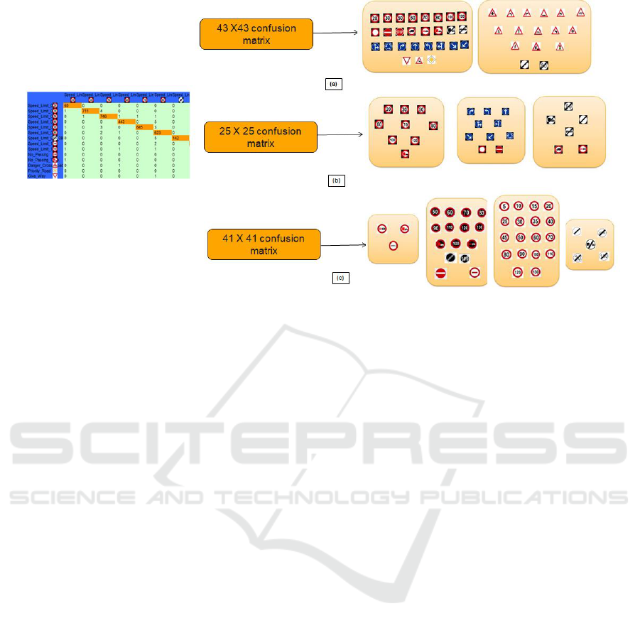
Figure 2: Spectral Clustering output for three cases. (a): Input is 43 × 43 confusion matrix. (b): Input is 25 × 25 confusion
matrix which is derived from confusion matrix in (a). (c): Input is 41 × 41 confusion matrix.
is 4. Speed Limit Inverse signs having black back-
ground and numeral written are grouped. Speed Limit
signs form the second group having the white back-
ground, red rim and numeral written. End signs form
the third group having white background and diago-
nal line crossing. Signs with pictogram and text form
another group having white background and red rim.
The parameters that can be tuned from outside are
sharpness parameter and epsilon.
4.2 Hierarchical Classification
Framework
This solution is designed for countries which signed
the Vienna Convention on Road Signs and Signals,
more particularly, European countries. The experi-
ments are done only on a subset of triangular signs
which are collected in-house. The dataset is prepared
by extracting the cutouts using box labels (x0, y0, x1,
y1). The cutouts obtained are of various sizes from
less than 10 × 10 pixels to greater than 100 × 100
pixels. Since the dataset is imbalanced (50 to 5000
images per class), image augmentation methods like
rotation (less than 15 degrees), zoom, and modifica-
tion of height and width are used to maintain a con-
stant number of samples across all classes. Train-
ing data contains both augmented and real sample
whereas the test data is taken from only the real sam-
ples. However the images taken in test data are from
videos having different track Id (identity) thereby en-
suring that model may not have seen those cutouts.
During training, the data is from different tracks. The
optimizer used is Adadelta which is more robust and
more powerful extension of Adagrad. The loss used
is categorical cross entropy. In the following sub-
sections details of experimentation done on triangular
traffic signs and GTSRB is discussed. The batch size
used in experiments is 50 and the number of epochs
are 40.
4.2.1 Triangular Sign Dataset
The first experiment done is on triangular traffic signs
which consists of both white and yellow background
signs. The total number of classes is 29 and the total
number of training samples are 28,789 with around
1000 samples in each class. The building block CNN
(flat classifier) is trained with an accuracy of 99.62%
and loss of 0.016. After training building block CNN,
validation data is applied to pre-trained building block
to get the confusion matrix. Validation data should
also be balanced. The total validation data tested is
5696 samples with around 300 samples for each class.
The accuracy of flat classifier obtained is 92.1%.
Now, spectral clustering algorithm is applied to this
confusion matrix to get disjoint many to one mapping.
The optimal number of clusters is automatically deter-
mined by the modified spectral clustering algorithm.
The mapping obtained is shown in Fig. 3 and thus,
two-level category hierarchy is automatically learned
by the model. As shown in figure, three groups are
formed. The first group consists of classes having
white background and the straight line in the middle
of the sign. The second group is formed based on
the background color and all the yellow background
classes are clustered in this group. And the last group
consists of white background signs similar to the first
ICPRAM 2020 - 9th International Conference on Pattern Recognition Applications and Methods
312

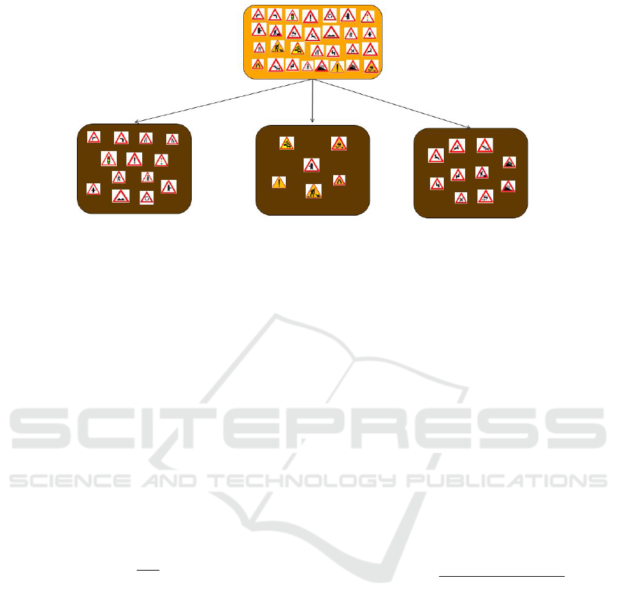
Figure 3: Category Hierarchy formed after spectral clustering for 29 class problem.
group but having an inclined line inside.
To get overlapped fine to coarse mapping the like-
lihood is calculated for each fine category. Based on
the likelihood of each class, categories which are hav-
ing a likelihood greater than the threshold for a par-
ticular coarse category is assigned to that coarse cat-
egory. Let M
d
i1
, M
d
i2
, .... M
d
iK
be the output of aggre-
gation layer by adding intermediate predictions M
f
i1
,
M
f
i2
, .... M
f
iC
for all those fine classes which belongs
to coarse class k based on disjoint many to one map-
ping P
d
. Here, 1 to C are total fine classes which are
clustered into K coarse groups.
M
d
ik
=
∑
j|P
d
( j)=k
M
f
i j
. (8)
Let u
1
( j), u
2
( j), u
3
( j), .... u
K
( j) be the likelihoods
for class j. The likelihood is given by,
u
k
( j) =
1



S
f
j



∑
i∈S
f
j
M
d
ik
. (9)
If u
k
( j) > threshold then fine category j is mapped
to coarse category k. Here, 1 ≤ j ≤ C and 1 ≤ k ≤ K.
Note that one particular j can be mapped to multi-
ple coarse classes. Thus, an overlapped fine to coarse
mapping P
o
is obtained giving final coarse classifier
predictions

M
o
ik

K
k=1
, where o denotes overlapped
map. The threshold used here is 0.02. Then, a
fine classifier
{
F
k
}
K
k=1
corresponding to each coarse
category is trained by the images belonging to that
particular classifier only. For triangular traffic sign
dataset, three fine classifiers are trained dedicatedly
using images corresponding to each coarse category
thereby learn class-specific features. Fine classifier-
0 is trained for triangular classes having white back-
ground and vertical edge in the middle of pictogram.
Fine classifier-1 is trained for yellow background
classes. Fine classifier-2 is trained for white back-
ground classes having inclined edge in the pictogram.
Let I be the set of indices for fine classes, I =
{
1,2,....,C
}
. I
k
is obtained based on overlapped fine
to coarse mapping where I
k
⊂ I such that P
o
(I
k
) = k.
The training images of classes having indices as el-
ement of I
k
, are used to train F
k
. F
k
which is dedi-
catedly trained for k
th
coarse group gives fine classi-
fier predictions as
n
M
f
k
i j
o
|
I
k
|
j=1
. The final fine classifier
probabilities are,
P
k
(y
i
/x
i
) =

M
f
k
i j
j ∈ I
k
0 otherwise
(10)
To get the final prediction of image, the weighted av-
erage of fine class prediction is taken, weighted by
their corresponding coarse category prediction by the
coarse classifier. Probabilistic averaging is given by,
p(y
i
= j | x
i
) =
∑
K
k=1
M
o
ik
P
k
(y
i
= j | x
i
)
∑
K
k=1
M
o
ik
. (11)
A case illustrating whole process is pictorially
shown in Fig. 4. The results of these steps are shown
by taking an example of the Danger Road Works
Right sign. It may be noted that the flat classifier
classified it wrongly as Danger Traffic Jam Right sign
whereas the hierarchical classifier correctly classify
it. Thus, accuracy is improved from 92.1% to 93.3%
because of the hierarchical architecture.
4.2.2 German Traffic Sign Recognition
Benchmark
The same experiment is repeated on the publicly
available GTSRB dataset. This dataset contains 43
German traffic sign classes. Unlike earlier dataset
which contains sign classes which are having trian-
gular shape only, the GTSRB dataset contains sign
Hierarchical Traffic Sign Recognition for Autonomous Driving
313

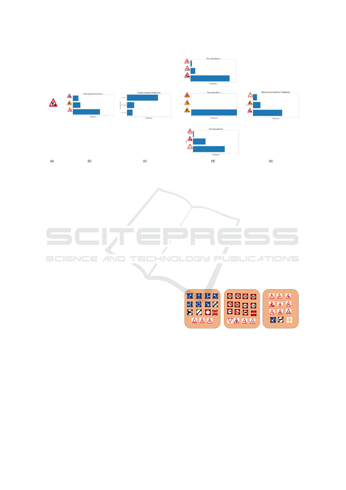
Figure 4: Case study on Triangular sign dataset.(a): Ground truth class of test image. (b): Top-3 predictions of flat classifier.
(c): Top-3 Coarse Classifier Predictions. (d): Top-3 Fine classifier predictions. (e): Top-3 Hierarchical Classifier Predictions.
classes which are both circular and triangular in
shapes. Thus, classes in this dataset can be easily dis-
tinguished as compared to the previous experiment of
only triangular sign classes. Training dataset is heav-
ily unbalanced from 210 to 2250 samples per class
and total 51,840 images with at least 30 images per
track. We maintained 1000 samples per class to train
the classifier ensuring that all the classes have equal
representative examples for training. The signs ob-
tained are of various sizes from 15 × 15 pixels to
222 × 193 pixels or more. In the earlier dataset,
groups were formed on the basis of color and pic-
togram inside the triangular shape. In this experi-
ment, the signs are of various shapes like circle, tri-
angle, quadrilateral, octagon and inverted triangular.
Therefore, this time even flat classifier will be able to
predict accurately because of large variation among
classes. However, still, there are few similarities be-
tween some sign classes. Thus, the hierarchy can be
obtained. The hierarchy and grouping obtained are
shown in Fig. 5 which is now on the basis of shape as
well as pictogram and background. The optimal num-
ber of clusters comes out to be 3 and the sign classes
are broadly grouped in 3 categories which are Direc-
tion signs, Speed Limit Signs and Danger Signs. It
is observed that the clustering done while learning
the category hierarchy have some errors. The rea-
son for this is that the category hierarchy is learned
by doing spectral clustering on the confusion matrix
formed using the validation data. The idea of spec-
tral clustering is that classes having some similarity
have high chances of getting confused and thus ex-
ploiting these confusions, similarity or affinity matrix
is obtained using confusion matrix. But in this case,
the building block classifier is performing really well
on validation data resulting in 99.6% accuracy. Thus,
most of the classes are accurately classified showing
no confusions with any of the class. Those classes can
be included in any of the group thus leading to mis-
takes in the grouping. The overall improvement of
accuracy on test data is from 98.7% to 99.0%. Thus,
our method outperforms the human performance on
GTSRB which is 98.8% (Stallkamp et al., 2012). The
images are misclassified due to motion blur, illumi-
nation variation, occlusion, and many other physical
factors. Thus, from these experiments, it can be seen
that the model can automatically detect the number of
clusters, learn the hierarchy, train the dedicated clas-
sifiers and thus improving the Top-1 classification ac-
curacy.
Figure 5: For GTSRB, clustering gives the optimal number
of clusters=3.
5 ANALYSIS
There are several issues which needs to be solved for
this particular work of hierarchical classification. The
first is an improvement in overall classification accu-
racy. Even though hierarchical classification is im-
proving the performance, it is observed that the dif-
ference in classification accuracy between flat and hi-
erarchical classifier is not as high as expected. We
ICPRAM 2020 - 9th International Conference on Pattern Recognition Applications and Methods
314

Algorithm 1: Two-level Hierarchical CNN Algo-
rithm.
Data: Dataset is
{
x
i
,y
i
}
where x
i
is image and
y
i
is the class label
Output: Final class prediction p (y
i
| x
i
) for
input image x
i
(1) Import, augment and pre-process the dataset.
(2) Split training set into the held-out set (sample
images from the training set randomly in such
a way that it have balanced class distribution)
and training set (remaining images). Dataset
has fine class labels for every image (labeled
from 1 to C) where C is total number of fine
categories.
(3) Single classifier training: Train flat classifier
(Building Block Net) to get C predictions
using the training set obtained above.
(4) Pass held-out set through trained building block
net and get predictions M
f
i j
where i denote
image index, j takes value from 1 to C and f
is a flag which denotes intermediate fine
predictions.
(5) Compute confusion matrix, F ∈ R
CXC
(6) Construct distance matrix,
D =
1
2
h
(I − F) + (I − F)
T
i
, (1)
with all diagonal entries set to zero.
(7) Convert distance matrix to similarity matrix
and use algorithm described in (Sanguinetti
et al., 2005) to estimate optimal value of
clusters K where K denotes number of coarse
categories.
(8) From Spectral Clustering algorithm (Ng et al.,
2002) the many to one mapping between fine
and coarse indices are obtained. The fine to
coarse mapping function is given as,
P
d
: I → S, (2)
where I =
{
1,2, ....C
}
and S =
{
1,2, ....K }
P
d
is a many to one function where d denotes
disjoint mapping. The function is defined as,
P
d
(I
k
) = k where I
k
⊂ I. (3)
I
k
is obtained based on spectral clustering
algorithm cluster assignments where k varies
from 1 to K. This means that all the fine
classes indexed by elements of I
k
are mapped
to the coarse class indexed by k.
(9) Evaluate M
d
ik
by aggregating intermediate fine
predictions M
f
i j
for all those fine classes which
belongs to coarse class k based on mapping
P
d
. In M
d
ik
, d is a flag denoting the aggregation
layer output based on disjoint mapping.
M
d
ik
=
∑
j|P
d
( j)=k
M
f
i j
. (4)
(10) Calculate the likelihood for each fine category
j which is given by,
u
k
( j) =
1



S
f
j



∑
i∈S
f
j
M
d
ik
, (5)
where
n
S
f
j
o
C
j=1
are fine class image
indicators. If u
k
( j) > threshold then fine
category j is mapped to coarse category k
where 1 ≤ k ≤ K. Note that one particular j
can be mapped to multiple coarse classes.
Thus, the overlapped fine to coarse mapping
P
o
is obtained where o denotes overlapped
map.
(11) Build single coarse classifier by adding fine to
coarse aggregation layer to give K output
predictions. Initialize weights by the weights
of pre-trained building block CNN because
both the front and end layers in the coarse
category component are similar to layers in
the building block CNN. Updated coarse
category predictions are
M
o
ik
=
∑
j|k∈P
o
( j)
M
i j
. (6)
Also, the predictions are `
1
normalized
because

M
o
ik

K
k=1
is greater than 1. In M
o
ik
, o
is a flag denoting the aggregation layer output
based on overlapped mapping.
(12) Build K fine classifiers for each coarse category
k. Output layer for each fine classifier will be
based on mapping P
o
. Train each fine
classifier, F
k
, in parallel using only image x
i
which belongs to coarse category k.
(13) Probabilistic Averaging:
p(y
i
= j | x
i
) =
∑
K
k=1
M
o
ik
P
k
(y
i
= j | x
i
)
∑
K
k=1
M
o
ik
. (7)
Hierarchical Traffic Sign Recognition for Autonomous Driving
315

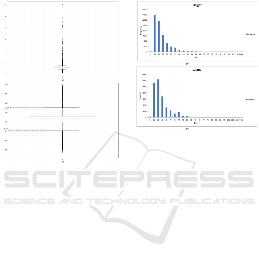
Figure 6: The box plot of aspect ratio for 29 class triangular
sign dataset with upper and lower thresholds. (a): Box plot.
(b): Zoomed version of box plot.
investigated into the reasons for this. Another prob-
lem is cutout sign variations from less than 10 × 10
pixels to greater than 100 × 100 pixels. Another op-
eration which can introduce errors is re-scaling of the
image using interpolation or downsizing. Yet another
issue is that the experiment is performed on the real-
time dataset. which means that the images captured
are of bad quality and have lots of variations due to
occlusions, illumination, scale, physical degradation
of sign boards, weather conditions, motion blur, etc.
These variations cause a decrease in accuracy because
some of the cutouts do not even contain any signs.
Thus, these outliers should be automatically detected
and removed. Also, some of the examples are misla-
beled. These wrong labels also results in a decrease
of accuracy. Thus, an analysis is required to be done
explore reasons for all the problems mentioned above.
5.1 Outliers Removal
In the case of real-time traffic signs, we observed that
in some bad images, only a little part of the sign is
there and no pictogram is actually visible. Thus, even
human will not be able to recognize this sign. These
outliers are typically captured by the camera when the
track is about to end and the last image which is cap-
Figure 7: The height and width histogram of 29 class trian-
gular sign dataset.
tured does not actually contain pictogram, however,
only the part of the traffic sign is visible. Removal of
these outliers will definitely boost the performance,
but manual removal of these outliers is a tedious task.
The outliers are eliminated by using box plot. The box
plot shows quartiles and interquartile which helps in
defining lower and upper bounds beyond which any
data point will be considered an outlier. In the case
of traffic signs, it is observed that the images which
are not having complete triangular signs have very
long height and small width or short height with a
very large width. The parameter which relates to both
height and width is aspect ratio which we use to re-
move the outliers. If the aspect ratio is either very
high or low, then the image is considered to be an
outlier. The thresholds (upper and lower) are fixed to
eliminate the outliers using a box plot. The box plot
of aspect ratio and its zoomed version for the origi-
nal 29 class traffic sign dataset is shown in Fig. 6.
The upper and lower threshold for removing the out-
liers are set as 1.38 and 0.77 as shown in the box plot.
While evaluating the pre-trained network, outliers are
removed from the data and an improvement in accu-
racy is noted from 92.4% to 93.8%. The improve-
ment is by 1.4%. Earlier, the accuracy was improved
from 92.1% to 93.3% where the improvement was by
1.2%.
ICPRAM 2020 - 9th International Conference on Pattern Recognition Applications and Methods
316

5.2 Size of Traffic Sign Images
Another serious issue which we noticed is the size of
the real-time traffic sign images. Even if the aspect
ratio is acceptable the size of image could be too low.
The dataset contains varying image sizes from lesser
than 10 × 10 pixels to greater than 100 × 100 pix-
els with varying aspect ratio. The histogram of height
and width of all the images in 29 class triangular sign
dataset is plotted as shown in Fig. 7. From the his-
togram, it is observed that most of the images are very
small in size and concentrated in the lower bins (0-
15). However, such tiny images do not contain any
useful information and after resizing to larger size im-
age that information is also lost. For example, an im-
age of size 1 × 4 contains only 4 pixels which are
not enough for classification. Also, very small size
images when resized to 64 × 64 which is desired in-
put for our CNN model, the pixels are interpolated
and thus the resized image obtained will not be hav-
ing the information required for classification. The
images having both width and height below 15 are ig-
nored. Thus, even if one dimension is greater than
15 the image is included. The minimum dimension is
obtained as 11 or 12 because any image having an as-
pect ratio less than 0.77 and greater than 1.38 is con-
sidered as an outlier. Thus, the minimum size image
possible now in the dataset is 11 × 15 pixels. After
removing all the tiny images from the dataset, eval-
uation is done on a pre-trained network. This shows
improvement in accuracy from 96.1% by the flat clas-
sifier to 96.9% by the hierarchical classifier. Earlier
it was just 93.3%. Thus, removing small size images
increase the accuracy of the classifier.
Another problem was resizing the image from
small sizes like 11 × 15 pixels to 64 × 64 pixels may
also lead to artifacts. A solution to this is spatial pyra-
mid matching (Gupta et al., 2018) which eliminates
the need for a fixed size input image. In this method,
original size images can be used. The limitation of
fixed size image in the input layer of CNN is because
of the fully connected layer at the end and not because
of convolution layers. We can get fixed length repre-
sentation from variable sized feature maps using this
concept. Table 3, shows feature map sizes for gen-
eral M × N × 3 image as input to our building block
CNN. It is observed that if we want at least 1 × 1 fea-
ture map to be present till the last layer the minimum
size of the image should be 22 × 22 × 3. However,
in our case, the smallest image size can be 11 × 15.
Thus, this concept cannot be used here.
5.3 Results after Removing both
Outliers and Small-sized Images
In this section, results are obtained by removing both
outliers and small sized images. After this step,
the count of training images become lesser than half
which is 14097 which means half of the images in
the dataset were small sized images. Also, the vali-
dation count falls to 2474 from 5948. The pre-trained
network is now evaluated by these 2474 images. The
result obtained is 96.7% accuracy by the flat classi-
fier and 97.5% accuracy by the hierarchical classifier
which is better than all the cases mentioned above.
It is observed that 62 examples are misclassified by
hierarchical classifier from total 2474 examples. Out
of these 62 examples around 50 examples cannot be
even correctly classified by the human. The reasons
for misclassification are complete and partial occlu-
sion, motion blur, scale variation, illumination varia-
tions, and label noise. Thus, the hierarchical classifier
performance of 97.5% accuracy is nearly justified.
5.4 Super-resolution
Resizing by interpolation reduces contrast (sharp
edges). It is desirable to recover finer texture details
when we upscale the image. Super-resolution tech-
nique is used to upscale the image to preserve per-
ceptual details. There are many different ways of up-
scaling the image by super-resolution. Some of those
methods are prediction based, image statistics based,
edge-preserving based, example pair-based methods
etc. Here, single image super-resolution is done using
Generative Adversarial Network (SRGAN) (Ledig
et al., 2017). Image scaling is required because build-
ing block CNN is taking a fixed size image as input
which is 64 × 64 × 3. The super-resolution tech-
nique is applied to 29 class triangular sign dataset for
upscaling small images by a factor of 4. The SRGAN
network is not trained from scratch instead a network
pre-trained for DIV2K dataset is used. It is observed
that the image upscaled using bicubic interpolation is
blurred whereas the super-resolved image is percep-
tually satisfying preserving texture details. To train
the network from scratch using super-resolved images
we have to restructure our dataset of 29 class triangu-
lar sign images. It is observed that after removing
small images and outliers, in one of the class there is
no example present in the validation set. Also, now
the training images are also very less which is 14097.
Thus, to train the model from scratch using super-
resolved images we have to restructure the dataset.
Heavy augmentation is done and now the validation
images contain different tracks of signs. In this case
Hierarchical Traffic Sign Recognition for Autonomous Driving
317

Table 3: Feature map size for M × N × 3 image as input to building block CNN.
Layer Configuration Feature map size
Input
b
M
c
×
b
N
c
× 3
Convolution 32, 3 × 3, same
b
M
c
×
b
N
c
× 32
Convolution 32, 3 × 3
b
M − 2
c
×
b
N − 2
c
× 32
Max Pooling 2 × 2
b
0.5M − 1
c
×
b
0.5N − 1
c
× 32
Dropout 0.2
Convolution 64, 3 × 3, same
b
0.5M − 1
c
×
b
0.5N − 1
c
× 64
Convolution 64, 3 × 3
b
0.5M − 3
c
×
b
0.5N − 3
c
× 64
Max Pooling 2 × 2
b
0.25M − 1.5
c
×
b
0.25N − 1.5
c
× 64
Dropout 0.2
Convolution 128, 3 × 3 filters, same
b
0.25M − 1.5
c
×
b
0.25N − 1.5
c
× 128
Convolution 128, 3 × 3
b
0.25M − 3.5
c
×
b
0.25N − 3.5
c
× 128
Max Pooling 2 × 2
b
0.125M − 1.75
c
×
b
0.125N − 1.75
c
× 128
Dropout 0.2
also the optimal number of clusters is three like the
previous cases. The accuracy of the flat classifier
is 95.0% which is increased to 97.3% by the hierar-
chical classifier which is a significant improvement.
This shows that accuracy depends on how the image
is resized. In this case also most of the examples are
wrongly classified because of motion blur, illumina-
tion variation and occlusion.
5.5 Comparison with State of Art
In this section, all the results are consolidated and
compared with the results present in the (Yan et al.,
2015). Table 4 tabulates the results obtained after
doing experimentation on various datasets. It is ob-
served that improvement in accuracy is in the range
of 0.3% to 2.3%. As the accuracy keeps on increas-
ing the improvement seems to be much lower. The
minimum improvement is reported when the building
block accuracy is maximum which is 98.7% for GT-
SRB dataset. Table 5 shows the state of art improve-
ments using hierarchical classifier. From the table it
is observed that, in (Yan et al., 2015) the improve-
ment is in the range of 0.9% to 3.6%. Here, consid-
ering the case of ImageNet testing, we observe that
the improvement i.e., the reduction in testing error
is maximum when the network is NIN and the base
network is giving high error. Whereas, when Ima-
geNet testing is done on VGG-16 network then the
base network error itself get reduced as compared to
NIN case, but the reduction in error from base to hier-
archical is low which is 0.96% only. Therefore, in this
case also, when the testing error of the base network
is already less then the improvement, i.e., that the re-
duction in testing error is low. Another advantage of
proposed solution is lesser number of computations
and trainable parameters due to shared layers and less
complex architecture. For GTSRB dataset, the train-
able parameters for hierarchical classifier architecture
is 10.4M which is lesser than 38.5M (Cirean et al.,
2012), 23.2M (Jin et al., 2014), 14.6M (Arcos-Garca
et al., 2018) and other existing solutions giving com-
parable performance.
6 CONCLUSIONS AND FUTURE
WORK
Traffic sign classification problem of uneven visual
variability of traffic signs is solved using deep learn-
ing based hierarchical classification design. Au-
tomatic determination of number of clusters while
learning category hierarchy using spectral clustering
on the confusion matrix of building block CNN has
been adopted. By employing hierarchical classifier,
accuracy has improved from 92.1% to 93.3% for Tri-
angular sign dataset. This is improved further by
addressing the issues of outliers and size of images
which has improved accuracy to 97.5%. The prob-
lem of upscaling by interpolation has been solved us-
ing super-resolution GAN leading to significant ac-
curacy improvement. GTSRB dataset is showing im-
provement in accuracy from 98.7% to 99.0% which is
better than human accuracy of 98.8%. Here, the im-
provement in accuracy for flat to hierarchical is low.
It is observed that when base classifier is giving high
accuracy then the improvement in accuracy by the hi-
erarchical classifier is less. Further improvement in
accuracy can be made by using modern features and
better CNN architecture for building block, chang-
ing the values of hyperparameters like overlapping
threshold, sharpness parameter, filter parameters, etc.
Re-sampling techniques can be used to solve the prob-
lem of unbalanced datasets. The challenge of cutout
size variations are also required to be handled. To
ICPRAM 2020 - 9th International Conference on Pattern Recognition Applications and Methods
318

Table 4: Results of Experimentation done on various different dataset. BB: Building Block, HC: Hierarchical Classifier.
Dataset Network Accuracy Improvement
BB HC
29-Triangular original VGG-8 92.1 93.3 1.2
outliers removed 92.4 93.8 1.4
small size removed 96.1 96.9 0.8
both removed 96.7 97.5 0.8
29-super-resolved Triangular both removed VGG-8 95.0 97.3 2.3
GTSRB VGG-8 98.7 99.0 0.3
Table 5: State of Art Results (Yan et al., 2015). BB: Building Block, HC: Hierarchical Classifier.
Dataset Network Testing Error Improvement
BB HC
CIFAR 100 Single view Testing NIN 37.29 34.36 2.93
Multi view Testing 35.27 33.33 1.94
ImageNet Single view Testing NIN 41.52 37.92 3.62
Multi view Testing 39.76 36.66 3.1
Single view Testing VGG-16 32.30 31.34 0.96
Multi view Testing 24.79 23.69 1.1
deal with real-time bad quality images pre-processing
techniques can be explored. A study of accuracy re-
duction due to label noise and possible solutions to
handle mislabeling need to be explored. Better aug-
mentation techniques and one shot learning can be ap-
plied if very less examples of the particular class are
available. The hierarchical classifier can be extended
to multiple levels in the future.
REFERENCES
Arcos-Garca, l., Alvarez-Garcia, J., and Soria Morillo, L.
(2018). Deep neural network for traffic sign recogni-
tion systems: An analysis of spatial transformers and
stochastic optimisation methods. Neural Networks,
99.
Cirean, D., Meier, U., Masci, J., and Schmidhuber, J.
(2012). Multi-column deep neural network for traf-
fic sign classification. Neural networks : the official
journal of the International Neural Network Society,
32:333–8.
Gavrila, D. M. (1998). Multi-feature hierarchical tem-
plate matching using distance transforms. In Proceed-
ings. Fourteenth International Conference on Pat-
tern Recognition (Cat. No.98EX170), volume 1, pages
439–444 vol.1.
Gupta, S., Pradhan, D. K., Dinesh, D. A., and Thenkanidiy-
oor, V. (2018). Deep spatial pyramid match kernel for
scene classification. In ICPRAM.
Jin, J., Fu, K., and Zhang, C. (2014). Traffic sign recogni-
tion with hinge loss trained convolutional neural net-
works. IEEE Transactions on Intelligent Transporta-
tion Systems, 15(5):1991–2000.
LeCun, Y., Haffner, P., Bottou, L., and Bengio, Y. (1999).
Object recognition with gradient-based learning. In
Shape, Contour and Grouping in Computer Vision,
pages 319–, London, UK, UK. Springer-Verlag.
Ledig, C., Theis, L., Huszr, F., Caballero, J., Cunningham,
A., Acosta, A., Aitken, A., Tejani, A., Totz, J., Wang,
Z., and Shi, W. (2017). Photo-realistic single image
super-resolution using a generative adversarial net-
work. In 2017 IEEE Conference on Computer Vision
and Pattern Recognition (CVPR), pages 105–114.
Ng, A. Y., Jordan, M. I., and Weiss, Y. (2002). On spectral
clustering: Analysis and an algorithm. In Dietterich,
T. G., Becker, S., and Ghahramani, Z., editors, Ad-
vances in Neural Information Processing Systems 14,
pages 849–856. MIT Press.
Sanguinetti, G., Laidler, J., and Lawrence, N. D. (2005).
Automatic determination of the number of clusters us-
ing spectral algorithms. In 2005 IEEE Workshop on
Machine Learning for Signal Processing, pages 55–
60.
Stallkamp, J., Schlipsing, M., Salmen, J., and Igel, C.
(2012). Man vs. computer: Benchmarking machine
learning algorithms for traffic sign recognition. Neu-
ral networks : the official journal of the International
Neural Network Society, 32:323–32.
Thrun, S. (2010). Toward robotic cars. Commun. ACM,
53(4):99–106.
Hierarchical Traffic Sign Recognition for Autonomous Driving
319

Vidal, R. (2011). Subspace clustering. IEEE Signal Pro-
cessing Magazine, 28(2):52–68.
Wang, G., Ren, G., Wu, Z., Zhao, Y., and Jiang, L. (2013).
A hierarchical method for traffic sign classification
with support vector machines. In The 2013 Interna-
tional Joint Conference on Neural Networks (IJCNN),
pages 1–6.
Xiao, T., Zhang, J., Yang, K., Peng, Y., and Zhang, Z.
(2014). Error-driven incremental learning in deep con-
volutional neural network for large-scale image clas-
sification. In ACM Multimedia.
Xuehong Mao, Hijazi, S., Casas, R., Kaul, P., Kumar, R.,
and Rowen, C. (2016). Hierarchical cnn for traffic
sign recognition. In 2016 IEEE Intelligent Vehicles
Symposium (IV), pages 130–135.
Yan, Z., Zhang, H., Piramuthu, R., Jagadeesh, V., DeCoste,
D., Di, W., and Yu, Y. (2015). Hd-cnn: Hierarchi-
cal deep convolutional neural networks for large scale
visual recognition. In The IEEE International Confer-
ence on Computer Vision (ICCV).
Zhu, X. and Bain, M. (2017). B-CNN: branch convolutional
neural network for hierarchical classification. CoRR,
abs/1709.09890.
ICPRAM 2020 - 9th International Conference on Pattern Recognition Applications and Methods
320