User-controllable Multi-texture Synthesis with Generative Adversarial

Networks

Aibek Alanov

1,2,3

, Max Kochurov

2,4

, Denis Volkhonskiy

, Daniil Yashkov

Evgeny Burnaev

and Dmitry Vetrov

2,3

National Research University Higher School of Economics, Moscow, Russia

Samsung AI Center Moscow, Moscow, Russia

Samsung-HSE Laboratory, National Research University Higher School of Economics, Moscow, Russia

Skolkovo Institute of Science and Technology, Moscow, Russia

Federal Research Center ”Computer Science and Control” of the Russian Academy of Sciences, Moscow, Russia

Keywords:

Texture Synthesis, Manifold Learning, Deep Learning, Generative Adversarial Networks.

Abstract:

We propose a novel multi-texture synthesis model based on generative adversarial networks (GANs) with a

user-controllable mechanism. The user control ability allows to explicitly specify the texture which should be

generated by the model. This property follows from using an encoder part which learns a latent representation

for each texture from the dataset. To ensure a dataset coverage, we use an adversarial loss function that

penalizes for incorrect reproductions of a given texture. In experiments, we show that our model can learn

descriptive texture manifolds for large datasets and from raw data such as a collection of high-resolution

photos. We show our unsupervised learning pipeline may help segmentation models. Moreover, we apply our

method to produce 3D textures and show that it outperforms existing baselines.

1 INTRODUCTION

Textures are essential and crucial perceptual elements

in computer graphics. They can be deﬁned as im-

ages with repetitive or periodic local patterns. Texture

synthesis models based on deep neural networks have

recently drawn a great interest to a computer vision

community. Gatys et al.(Gatys et al., 2015; Gatys

et al., 2016b) proposed to use a convolutional neu-

ral network as an effective texture feature extractor.

They proposed to use a Gram matrix of hidden layers

of a pre-trained VGG network as a descriptor of a tex-

ture. Follow-up papers (Johnson et al., 2016; Ulyanov

et al., 2016) signiﬁcantly speed up a synthesis of tex-

ture by substituting an expensive optimization process

in (Gatys et al., 2015; Gatys et al., 2016b) to a fast for-

ward pass of a feed-forward convolutional network.

However, these methods suffer from many problems

such as generality inefﬁciency (i.e., train one network

per texture) and poor diversity (i.e., synthesize visu-

ally indistinguishable textures).

Recently, Periodic Spatial GAN (PSGAN)

(Bergmann et al., 2017) and Diversiﬁed Texture Syn-

thesis (DTS) (Li et al., 2017) models were proposed

Figure 1: One can take 1) New Guinea 3264 × 4928 landscape photo, learn 2) a manifold of 2D texture embeddings for this

photo, visualize 3) texture map for the image and perform 4) texture detection for a patch using distances between learned

embeddings.

First two authors have equal contribution.

214

Alanov, A., Kochurov, M., Volkhonskiy, D., Yashkov, D., Burnaev, E. and Vetrov, D.

User-controllable Multi-texture Synthesis with Generative Adversarial Networks.

DOI: 10.5220/0008924502140221

In Proceedings of the 15th International Joint Conference on Computer Vision, Imaging and Computer Graphics Theory and Applications (VISIGRAPP 2020) - Volume 4: VISAPP, pages

214-221

ISBN: 978-989-758-402-2; ISSN: 2184-4321

Legend

- encoder

- generator

- texture pair  

        discriminator

- texture        

     discriminator

- latent         

     discriminator

Prior distribution

sample

Texture sample

Prior distribution

sample

Same texture

samples

Fake Real

Texture sample

Pair

Matching

Generation

Matching

Encoder

Matching

Texture sample

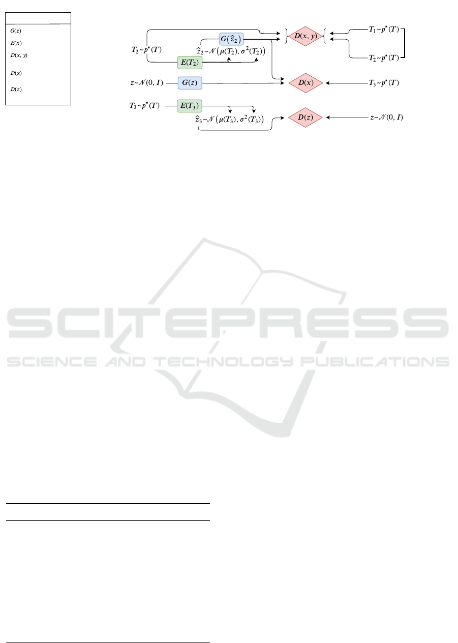
Figure 2: Training pipeline of the proposed method.

as an attempt to partly solve these issues. PSGAN

and DTS are multi-texture synthesis models, i.e.,

they train one network for generating many textures.

However, each model has its own limitations (see

Table 1). PSGAN has incomplete dataset coverage,

and a user control mechanism is absent. Lack of

dataset coverage means that it can miss some textures

from the training dataset. The absence of a user

control does not allow to explicitly specify the texture

which should be generated by the model in PSGAN.

DTS is not scalable with respect to dataset size,

cannot be applied to learn textures from raw data and

to synthesize 3D textures. It is not scalable because

the number of parameters of the DTS model linearly

depends on the number of textures in the dataset. The

learning from raw data means that the input for the

model is a high-resolution image as in Figure 1 and

the method should extract textures in an unsupervised

way. DTS does not support such training mode

(which we call fully unsupervised) because for this

model input textures should be speciﬁed explicitly.

The shortage of generality to 3D textures in DTS

model comes from inapplicability of VGG network

to 3D images.

We propose a novel multi-texture synthesis model

which does not have limitations of PSGAN and DTS.

Table 1: Comparison of multi-texture synthesis methods.

PSGAN DTS Ours

multi-texture X X X

user control X X

dataset coverage X X

scalability with respect

to dataset size

X X

ability to learn textures

from raw data

X X

unsupervised texture

detection

applicability to 3D X X

Our model allows for generating a user-speciﬁed tex-

ture from the training dataset. This is achieved by

using an encoder network which learns a latent repre-

sentation for each texture from the dataset. To ensure

the complete dataset coverage of our method we use

a loss function that penalizes for incorrect reproduc-

tions of a given texture. Thus, the generator is forced

to learn the ability to synthesize each texture seen dur-

ing the training phase. Our method is more scalable

with respect to dataset size compared to DTS and is

able to learn textures in a fully unsupervised way from

raw data as a collection of high-resolution photos. We

show that our model learns a descriptive texture mani-

fold in latent space. Such low dimensional representa-

tions can be applied as useful texture descriptors, for

example, for an unsupervised texture detection (see

Figure 1) or improving segmentation models. Also,

we can apply our approach to 3D texture synthesis be-

cause we use fully adversarial losses and do not utilize

VGG network descriptors.

We experimentally show that our model can learn

large datasets of textures. We check that our generator

learns all textures from the training dataset by condi-

tionally synthesizing each of them. We demonstrate

that our model can learn meaningful texture mani-

folds as opposed to PSGAN (see Figure 6). We com-

pare the efﬁciency of our approach and DTS in terms

of memory consumption and show that our model is

much more scalable than DTS for large datasets. We

also provide proof of concept experiments showing

that embeddings learned in an unsupervized way may

help segmentation models.

We apply our method to 3D texture-like porous

media structures which is a real-world problem from

Digital Rock Physics. Synthesis of porous structures

plays an important role (Volkhonskiy et al., 2019) be-

cause an assessment of the variability in the inherent

material properties is often experimentally not feasi-

ble. Moreover, usually it is necessary to acquire a

number of representative samples of the void-solid

User-controllable Multi-texture Synthesis with Generative Adversarial Networks

215

structure. We show that our method outperforms a

baseline (Mosser et al., 2017) in the porous media

synthesis which trains one network per texture.

Brieﬂy summarize, we can highlight the following

key advantages of our model:

• user control (conditional generation),

• full dataset coverage,

• scalability with respect to dataset size,

• ability to learn descriptive texture manifolds from

raw data in a fully unsupervised way,

• applicability to 3D texture synthesis.

2 PROPOSED METHOD

We look for a multi-texture synthesis pipeline that can

generate textures in a user-controllable manner, en-

sure full dataset coverage and be scalable with respect

to dataset size. We use an encoder network E

(x)

which allows to map textures to a latent space and

gives low dimensional representations. We use a sim-

ilar generator network G

(z) as in PSGAN.

The generator G

(z) takes as an input a noise ten-

sor z ∈ R

d×h

×w

which has three parts z = [z

, z

These parts are the same as in PSGAN:

• z

∈ R

×h

×w

is a global part which determines

the type of texture. It consists of only one vec-

tor ¯z

of size d

which is repeated through spatial

dimensions.

• z

∈ R

×h

×w

is a local part and each element

ki j

is sampled from a standard normal distribu-

tion N (0, 1) independently. This part encourages

the diversity within one texture.

• z

∈ R

×h

×w

is a periodic part and z

ki j

sin(a

) · i + b

) · j + ξ

) where a

, b

are

trainable functions and ξ

is sampled from

U[0, 2π] independently. This part helps generat-

ing periodic patterns.

We see that for generating a texture it is sufﬁcient

to put the vector ¯z

as an input to the generator G

be-

cause z

is obtained independently from N (0, 1) and

is computed from z

. It means that we can consider

¯z

as a latent representation of a corresponding texture

and we will train our encoder E

(x) to recover this la-

tent vector ¯z

for an input texture x. Further, we will

assume that the generator G

(z) takes only the vector

¯z

as input and builds other parts of the noise tensor

from it. For simplicity, we denote ¯z

as z.

The encoder E

(x) takes an input texture x and

returns the distribution q

(z|x) = N (µ

(x), σ

(x)) of

the global vector z (the same as ¯z

) of the texture x.

Then we can formulate properties of the generator

(z) and the encoder E

(x) we expect in our model:

• samples G

(z) are real textures if we sample z

from a prior p(z) (in our case it is N (0, I)).

• if z

(x) ∼ q

(z|x) then G

(x)) has the same

texture type as x.

• an aggregated distribution of the encoder E

(x)

should be close to the prior p(z), i.e. q

(z) =

(z|x)p

∗

(x)dx ≈ p(z) where p

∗

(x) is a true dis-

tribution of textures.

• samples G

) are real textures if z

is sampled

from aggregated q

(z).

To ensure these properties we use three types of

adversarial losses:

• generator matching: L

for matching the distri-

bution of both samples G

(z) and reproductions

) to the distribution of real textures p

∗

(x).

• pair matching: L

for matching the distribu-

tion of pairs (x, x

) to the distribution of pairs

(x, G

(x))) where x and x

are samples of the

same texture. It will ensure that G

(x)) has the

same texture type as x.

• encoder matching: L

for matching the aggre-

gated distribution q

(z) to the prior p(z).

We consider exact deﬁnitions of these adversar-

ial losses in Section 2.1. We demonstrate the whole

pipeline of the training procedure in Figure 2.

2.1 Generator & Encoder Objectives

Generator Matching. For matching both samples

(z) and reproductions G

) to real textures we

use a discriminator D

(x) as in PSGAN which maps

an input image x to a two-dimensional tensor of spa-

tial size s × t. Each element D

i j

(x) of the discrimi-

nator’s output corresponds to a local part x and esti-

mates probability that such receptive ﬁeld is real ver-

sus synthesized by G

. Then a value function V

(θ, ψ)

of such adversarial game min

max

(θ, ψ) will be the

following:

(θ, ψ) =

s,t

∑

i, j

∗

(x)

logD

i j

(x) (1)

p(z)

log(1 − D

i j

(z)))

+ E

(z)

log(1 − D

i j

)))

As in (Goodfellow et al., 2014) we modify the

value function V

(θ, ψ) for the generator G

by sub-

stituting the term log(1 − D

i j

(·)) to − log D

i j

(·). So,

VISAPP 2020 - 15th International Conference on Computer Vision Theory and Applications

216

image 1

image 2

conv1x1 + ReLU + conv1x1

logits 1 logits 2

Figure 3: The architecture of the discriminator on pairs D

(x, y).

the adversarial loss L

(θ) = −

s,t

∑

i, j

p(z)

logD

i j

(z))+ (2)

(z)

logD

i j

))

→ min

Pair Matching. The goal is to match fake pairs

(x, G

(x))) to real ones (x, x

) where x and x

are

samples of the same texture (in practice, we can ob-

tain real pairs by taking two different random patches

from one texture). For this purpose we use a discrim-

inator D

(x, y) of special architecture which is pro-

vided in Figure 3.

We consider the following distributions:

• p

∗

(x, y) over real pairs (x, y) where x and y are

examples of the same texture;

• p

θ,ϕ

(x, y) over fake pairs (x, y) where x is a

real texture and y is its reproduction, i.e., y =

(x)).

We denote the dimension of the discriminator’s

output matrix as p × q and D

i j

(x, y) as the i j-th ele-

ment of this matrix. The value function V

(θ, ϕ, τ)

for this adversarial game min

θ,ϕ

max

(θ, ϕ, τ) is

(θ, ϕ, τ) =

p,q

∑

i, j

∗

(x,y)

logD

i j

(x, y) +

+ E

θ,ϕ

(x,y)

log(1 − D

i j

(x, y))

(3)

The discriminator D

tries to maximize the value

function V

(θ, ϕ, τ) while the generator G

and the

encoder E

minimize it.

Then the adversarial loss L

(θ, ϕ) = −

p,q

∑

i, j

θ,ϕ

(x,y)

logD

i j

(x, y) → min

θ,ϕ

(4)

Encoder Matching. We need to use encoder match-

ing because otherwise if we use only one objective

(θ, ϕ) for training the encoder E

(x) then embed-

dings for textures can be very far from samples z that

come from the prior distribution p(z). It will lead

to unstable training of the generator G

(z) because it

should generate good images both for samples from

the prior p(z) and for embeddings which come from

the encoder E

Therefore, to regularize the encoder E

we match

the prior distribution p(z) and the aggregated encoder

distribution q

(z) =

(z|x)p

∗

(x)dx using the dis-

criminator D

(z). It classiﬁes samples z from p(z)

versus ones from q

(z). The minimax game of E

(x)

and D

is deﬁned as min

max

(ϕ, ζ), where V

(ϕ, ζ)

(ϕ, ζ) = E

p(z)

logD

(z) (5)

(z)

log(1 − D

(z))

To sample from q

(z) we should at ﬁrst sample some

texture x then sample z from the encoder distribution

by z = µ

(x) + σ

(x) ∗ ε, where ε ∼ N (0, I). The ad-

versarial loss L

(ϕ) is

(ϕ) = −E

(z)

logD

(z) → min

(6)

Final Objectives. Thus, for both the generator G

and the encoder E

we optimize the following objec-

tives:

• the generator G

loss

L(θ) = α

(θ) + α

(θ, ϕ) → min

(7)

• the encoder E

loss

L(ϕ) = β

(ϕ) + β

(θ, ϕ) → min

(8)

In experiments, we use α

= α

= β

= 1.

3 RELATED WORK

Deep learning methods were shown to be an efﬁcient

parametric model for texture synthesis. Papers of

Gatys et al.(Gatys et al., 2015; Gatys et al., 2016b)

are a milestone: they proposed to use Gram matrices

of VGG intermediate layer activations as texture de-

scriptors. This approach allows for generating high-

quality images of textures (Gatys et al., 2015) by

User-controllable Multi-texture Synthesis with Generative Adversarial Networks

217

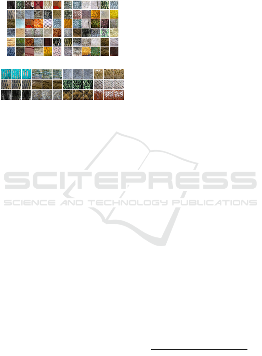
(a) PSGAN-5D samples (b) Our-2D model samples

textures, others are reproductions

Figure 4: Examples of generated/reproduced textures from

PSGAN and our model.

running an expensive optimization process. Subse-

quent works (Ulyanov et al., 2016; Johnson et al.,

2016) signiﬁcantly accelerate a texture synthesis by

approximating this optimization procedure by fast

feed-forward convolutional networks. Further works

improve this approach either by using optimization

techniques (Frigo et al., 2016; Gatys et al., 2016a;

Li and Wand, 2016), introducing an instance normal-

ization (Ulyanov et al., 2017; Ulyanov et al., ) or ap-

plying GANs-based models for non-stationary texture

synthesis (Zhou et al., 2018). These methods have

signiﬁcant limitations such as the requirement to train

one network per texture and poor diversity of samples.

Multi-texture Synthesis Methods. DTS (Li et al.,

2017) was introduced by Li et al.as a multi-texture

synthesis model. Spatial GAN (SGAN) model

(Jetchev et al., 2016) was introduced by Jetchev

et al.as the ﬁrst method where GANs are applied to

texture synthesis. It showed good results, surpass-

ing the results of (Gatys et al., 2015). Bergmann

et al.(Bergmann et al., 2017) improved SGAN by in-

troducing Periodic Spatial GAN (PSGAN) model.

Our model is based on GANs with an encoder net-

work which allows mapping an input texture to a la-

tent embedding. We use the adversarial loss for this

purpose inspired by (Xian et al., 2018) where it is

used for image synthesis guided by sketch, color, and

texture. The beneﬁt of such loss is that it can be eas-

ily applied to 3D textures. Previous works (Mosser

et al., 2017; Volkhonskiy et al., 2019) on synthesiz-

ing 3D porous material used GANs with 3D convolu-

tional layers inside a generator and a discriminator.

4 EXPERIMENTS

In experiments, we train our model on scaly, braided,

honeycomb and striped categories from Oxford De-

scribable Textures Dataset (Cimpoi et al., 2014).

These are datasets with natural textures in the wild.

We use the same fully-convolutional architecture for

(x), G

(z) as in PSGAN (Bergmann et al., 2017).

We used a spectral normalization (Miyato et al., 2018)

for discriminators that signiﬁcantly improved training

stability.

4.1 Inception Score for Textures

It is a common practice in natural image generation

to evaluate a model that approximates data distri-

bution p

∗

(x) using Inception Score (Szegedy et al.,

2016). For this purpose Inception network is used

to get label distribution p(t|x). Then one calculates

IS = exp



x∼p

∗

(x)



p(t|x)kp(t)



, where p(t) =

x∼p

∗

(x)

p(t|x) is aggregated label distribution. The

straightforward application of Inception network does

not make sense for textures. Therefore, we train a

classiﬁer with an architecture similar

∗

to D

(x) to

predict texture types for a given texture dataset. To do

that properly, we manually clean our data from dupli-

cates so that every texture example has a distinct label

and use random cropping as data augmentation. Our

trained classiﬁer achieves 100% accuracy on a scaly

dataset. We use this classiﬁer to evaluate Inception

Score for models trained on the same texture dataset.

4.2 Unconditional and Conditional

Generation

For models like PSGAN we are not able to obtain re-

productions, we only have access to texture genera-

tion process. One would ask for the guarantees that a

model is able to generate every texture in the dataset

from only the prior distribution. We evaluate PSGAN

and our model on a scaly dataset with 116 unique tex-

tures. After models are trained, we estimate the In-

ception Score. We observed that Inception Score dif-

Table 2: Inception Scores for conditional and unconditional

generation from PSGAN and our model. Classiﬁer used to

compute IS achieved perfect accuracy on train data.

Model Uncond. IS Cond. IS

PSGAN-5D 73.68±0.6 NA

Our-2D 73.74±0.3 103.96±0.1

∗

The only difference is the number of output logits

VISAPP 2020 - 15th International Conference on Computer Vision Theory and Applications

218

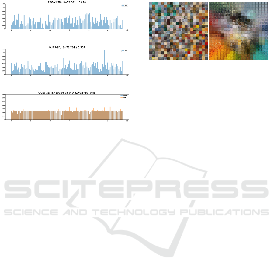
(a) PSGAN-5D samples

(b) Our-2D model samples

Figure 5: Histogram of classiﬁer predictions on 50000 gen-

erated samples from PSGAN (a) and Our model (b) and for

500 reproductions per class for our model (c). Each bin rep-

resents a separate texture class from scaly dataset.

fers with d

and thus picked the best d

separately

for both PSGAN and our model obtaining d

= 5

and d

= 2 respectively. Both models were trained

with Adam (Kingma and Ba, 2015) (betas=0.5,0.99)

with batch size 64 on a single GPU. Their best per-

formance was achieved in around 80k iterations. For

both models, we used spectral normalization to im-

prove training stability (Miyato et al., 2018).

Both models can generate high-quality textures

from low dimensional space. Our model additionally

can successfully generate reproductions for every tex-

ture in the dataset. Figure 5 and Table 2 summarise

the results for conditional (reproductions) and uncon-

ditional texture generation. Figure 5a indicates PS-

GAN may have missing textures, our model does not

suffer from this issue. Inception Score suggests that

conditional generation is a far better way to sample

from the model. In Figure 4 we provide samples and

texture reproductions for trained models.

4.3 Texture Manifold

Autoencoding property is a nice to have feature for

generative models. One can treat embeddings as low

dimensional data representations. As shown in sec-

tion 4.2 our model can reconstruct every texture in

the dataset. Moreover, we are able to visualize the

manifold of textures since we trained this model with

= 2. To compare this manifold to PSGAN, we train

a separate PSGAN model with d

= 2. 2D manifolds

(a) PSGAN 2D manifold (b) Ours 2D manifold

Figure 6: 2D manifold for 116 textures from scaly dataset.

Our model gives paces one texture to a distinct location.

Grid is taken over [−2.25, 2.25] × [−2.25, 2.25] with step

0.225.

near prior distribution for both models can be found

in Figure 6. Our model learns visually better 2D man-

ifold and allocates similar textures nearby.

4.4 Spatial Embeddings Structure

As described in sections 4.5 and 4.3, our method can

learn descriptive texture manifold from a collection

of raw data in an unsupervised way. The obtained

texture embeddings may be useful. Consider a large

input image X, e.g.as the ﬁrst in Figure 1, and the

trained G(z) and E(x) on this image. Note that at

the training stage encoder E(x) is a fully convolu-

tional network, followed by global average pooling.

Applied to X as-is, the encoder’s output would be

”average” texture embedding for the whole image X.

Replacing global average pooling by spatial average

pooling with small kernel allows E(X ) to output tex-

ture embeddings for each receptive ﬁeld in the input

image X. We denote such modiﬁed encoder as

E(x).

Z =

E(X) is a tensor with spatial texture embed-

dings for X. They smoothly change along spatial di-

mensions as visualized by reconstructing them with

generator

G(Z) on the third picture in Figure 1.

One can take a reference patch P with a texture

(e.g., grass) and ﬁnd similar textures in image X. This

is illustrated in the last picture in Figure 1. We picked

a patch P with grass on it and constructed a heatmap

M: M

i j

= exp(−αd(

E(X)

i j

, E(P))

), where d(·, ·) is

Euclidean distance and α = 3 in our example. We

then interpolated M to the original size of X.

This example shows that

E(x) allows using

learned embeddings for other tasks that have no re-

lation to texture generation. We believe supervised

methods would beneﬁt from adding additional fea-

tures obtained in an unsupervised way.

User-controllable Multi-texture Synthesis with Generative Adversarial Networks

219

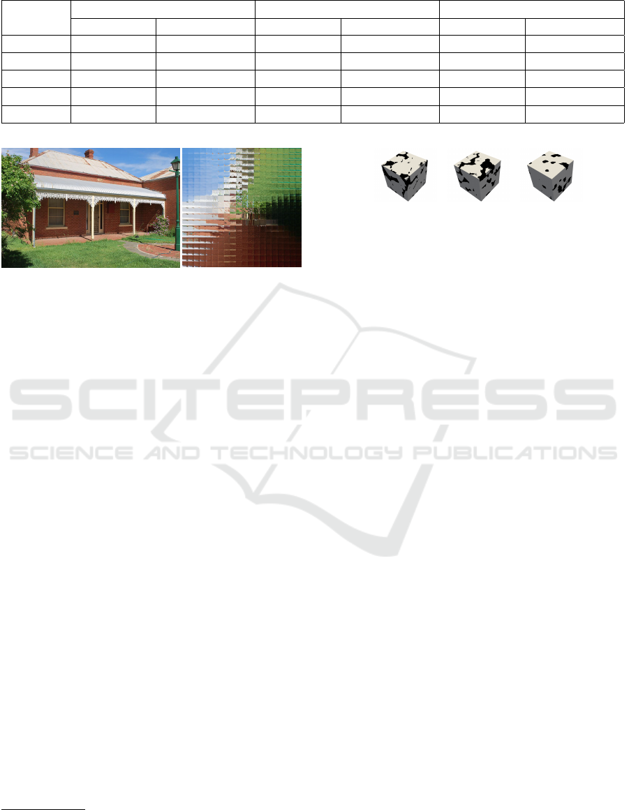
Table 3: KL divergence between real, our and the baseline distributions of statistics (permeability, Euler characteristic, and

surface area) for size 160

. The standard deviation was computed using the bootstrap method with 1000 resamples.

Permeability Euler characteristic Surface area

KL(p

real

, p

ours

) KL (p

real

, p

baseline

) KL (p

real

, p

ours

) KL (p

real

, p

baseline

) KL (p

real

, p

ours

) KL (p

real

, p

baseline

)

Ketton 5.06 ± 0.35 4.68 ± 0.56 3.66 ± 0.73 1.86 ± 0.42 1.85 ± 0.62 7.73 ± 0.18

Berea 0.49 ± 0.07 0.50 ± 0.12 0.34 ± 0.08 1.36 ± 0.25 0.33 ± 0.11 5.91 ± 0.54

Doddington 0.42 ± 0.10 3.41 ± 1.68 2.65 ± 2.29 3.35 ± 1.13 4.83 ± 2.06 7.92 ± 0.27

Estaillades 0.80 ± 0.24 3.41 ± 0.46 1.85 ± 0.29 2.05 ± 1.05 4.62 ± 0.66 6.93 ± 0.39

Bentheimer 0.47 ± 0.08 1.38 ± 0.49 1.24 ± 0.41 3.44 ± 1.91 1.20 ± 0.73 1.25 ± 0.12

Figure 7: Merrigum House 3872 × 2592 photo and its

learned 2D texture manifold using our model.

4.5 Learning Texture Manifolds from

Raw Data and Texture Detection

The learned manifold in section 4.3 was obtained

from well prepared data and a single image in sec-

tion 4.4. Real cases usually do not have clean data

and require either expensive data preparation or un-

supervised methods. Our model can learn texture

manifolds from raw data such as a collection of high-

resolution photos. To cope with training texture man-

ifolds on raw data, we suggest to construct p

∗

(x, x

) in

equation 3 with two crops from almost the same loca-

tion. In Figure 7 we provide a manifold learned from

House photo.

4.6 Application to 3D Synthesis

In this section, we demonstrate the applicability of our

model to the Digital Rock Physics. We trained our

model on 3D Porous Media structures

†

(i.e. see Fig.

8a) of ﬁve different types: Ketton, Berea, Dodding-

ton, Estaillades and Bentheimer. Each type of rock

has an initial size 1000

binary voxels. As the base-

line, we considered Porous Media GANs (Mosser

et al., 2017), which is deep convolutional GANs with

3D convolutional layers.

For the comparison of our model with real sam-

ples and the baseline samples, we use permeability

statistics and two so-called Minkowski functionals.

†

All samples were taken from Imperial College

database

(a) Real (b) Ours (c) Baseline

Figure 8: Real, synthetic (our model) and synthetic (base-

line model) Berea samples of size 150

We used the following experimental setup. We

trained our model on random crops of size 160

all types of porous structures. We also trained ﬁve

baseline models on each type separately. Then we

generated 500 synthetic samples of size 160

of each

type using our model and the baseline model. We also

cropped 500 samples of size 160

from the real data.

As a result, for each type of structure, we obtained

three sets of objects: real, synthetic and baseline.

The visual result of the synthesis is presented in

Fig. 8 for Berea. In the ﬁgure, there are three sam-

ples: real (i.e., cropped from the original big sample),

ours and a sample of the baseline model. Because our

model is fully convolutional, we can increase the gen-

erated sample size by expanding the spatial dimen-

sions of the latent embedding z. The network struc-

ture allows to produce larger texture sizes.Then, for

each real, synthetic and baseline objects we calculated

three statistics: permeability, Surface Area and Euler

characteristics. To measure the distance between dis-

tributions of statistics for real, our and baseline sam-

ples we approximated these distributions by discrete

ones obtained using the histogram method with 50

bins. Then for each statistic, we calculated KL diver-

gence between the distributions of the statistic of a)

real and our generated samples; b) real and baseline

generated samples.

The comparison of the KL is presented at Tab. 3

for the permeability and for Minkowski functionals.

As we can see, our model performs better accordingly

for most types of porous structures.

VISAPP 2020 - 15th International Conference on Computer Vision Theory and Applications

220

5 CONCLUSIONS AND FUTURE

WORK

In this paper, we proposed a novel model for multi-

texture synthesis. We showed it ensures full dataset

coverage and can detect textures on images in the un-

supervised setting. We provided a way to learn a man-

ifold of training textures even from a collection of raw

high-resolution photos. We also demonstrated that the

proposed model applies to the real-world 3D texture

synthesis problem: porous media generation. Our

model outperforms the baseline by better reproduc-

ing physical properties of real data. In future work,

we want to study the texture detection ability of our

model for improving segmentation in an unsupervised

way and seek for its new applications.

ACKNOWLEDGEMENTS

Aibek Alanov, Max Kochurov, Dmitry Vetrov were

supported by Samsung Research, Samsung Electron-

ics. The work of Dmitry Vetrov was supported by the

Russian Science Foundation grant no.17-71-20072.

The work of E. Burnaev and D. Volkhonskiy was sup-

ported by the MES of RF, grant No. 14.615.21.0004,

grant code: RFMEFI61518X0004. The authors E.

Burnaev and D. Volkhonskiy acknowledge the usage

of the Skoltech CDISE HPC cluster Zhores for ob-

taining some results presented in this paper.

REFERENCES

Bergmann, U., Jetchev, N., and Vollgraf, R. (2017). Learn-

ing texture manifolds with the periodic spatial gan.

ICML.

Cimpoi, M., Maji, S., Kokkinos, I., Mohamed, S., and

Vedaldi, A. (2014). Describing textures in the wild.

In Proc. IEEE CVPR, pages 3606–3613, Washington,

DC, USA. IEEE Computer Society.

Frigo, O., Sabater, N., Delon, J., and Hellier, P. (2016). Split

and match: Example-based adaptive patch sampling

for unsupervised style transfer. In Proc. IEEE CVPR,

pages 553–561.

Gatys, L., Ecker, A. S., and Bethge, M. (2015). Texture syn-

thesis using convolutional neural networks. In NIPS,

pages 262–270.

Gatys, L. A., Bethge, M., Hertzmann, A., and Shechtman,

E. (2016a). Preserving color in neural artistic style

transfer. arXiv preprint arXiv:1606.05897.

Gatys, L. A., Ecker, A. S., and Bethge, M. (2016b). Image

style transfer using convolutional neural networks. In

Proc. IEEE CVPR, pages 2414–2423.

Goodfellow, I., Pouget-Abadie, J., Mirza, M., Xu, B.,

Warde-Farley, D., Ozair, S., Courville, A., and Ben-

gio, Y. (2014). Generative adversarial nets. In NIPS,

pages 2672–2680.

Jetchev, N., Bergmann, U., and Vollgraf, R. (2016). Texture

synthesis with spatial generative adversarial networks.

arXiv preprint arXiv:1611.08207.

Johnson, J., Alahi, A., and Fei-Fei, L. (2016). Perceptual

losses for real-time style transfer and super-resolution.

In ECCV, pages 694–711. Springer.

Kingma, D. P. and Ba, J. (2015). Adam: A method for

stochastic optimization. In International Conference

on Learning Representations (ICLR).

Li, C. and Wand, M. (2016). Combining markov random

ﬁelds and convolutional neural networks for image

synthesis. In Proceedings of the IEEE Conference

on Computer Vision and Pattern Recognition, pages

2479–2486.

Li, Y., Fang, C., Yang, J., Wang, Z., Lu, X., and Yang,

M.-H. (2017). Diversiﬁed texture synthesis with feed-

forward networks. In Proc. CVPR.

Miyato, T., Kataoka, T., Koyama, M., and Yoshida, Y.

(2018). Spectral normalization for generative adver-

sarial networks. ICLR.

Mosser, L., Dubrule, O., and Blunt, M. J. (2017). Re-

construction of three-dimensional porous media using

generative adversarial neural networks. Physical Re-

view E, 96(4):043309.

Szegedy, C., Vanhoucke, V., Ioffe, S., Shlens, J., and Wojna,

Z. (2016). Rethinking the inception architecture for

computer vision. In 2016 IEEE Conference on Com-

puter Vision and Pattern Recognition, CVPR 2016,

Las Vegas, NV, USA, June 27-30, 2016, pages 2818–

2826.

Ulyanov, D., Lebedev, V., Vedaldi, A., and Lempitsky, V. S.

(2016). Texture networks: Feed-forward synthesis of

textures and stylized images. In ICML, pages 1349–

1357.

Ulyanov, D., Vedaldi, A., and Lempitsky, V. Instance nor-

malization: the missing ingredient for fast stylization.

corr abs/1607.0 (2016).

Ulyanov, D., Vedaldi, A., and Lempitsky, V. (2017). Im-

proved texture networks: Maximizing quality and di-

versity in feed-forward stylization and texture synthe-

sis. In Proceedings of the IEEE Conference on Com-

puter Vision and Pattern Recognition, pages 6924–

6932.

Volkhonskiy, D., Muravleva, E., Sudakov, O., Orlov, D.,

Belozerov, B., Burnaev, E., and Koroteev, D. (2019).

Reconstruction of 3d porous media from 2d slices.

arXiv preprint arXiv:1901.10233.

Xian, W., Sangkloy, P., Agrawal, V., Raj, A., Lu, J., Fang,

C., Yu, F., and Hays, J. (2018). Texturegan: Con-

trolling deep image synthesis with texture patches. In

Proceedings of the IEEE Conference on Computer Vi-

sion and Pattern Recognition, pages 8456–8465.

Zhou, Y., Zhu, Z., Bai, X., Lischinski, D., Cohen-Or,

D., and Huang, H. (2018). Non-stationary texture

synthesis by adversarial expansion. arXiv preprint

arXiv:1805.04487.

User-controllable Multi-texture Synthesis with Generative Adversarial Networks

221