An Autoregressive Multiple Model Probabilistic Framework for the

Detection of SSVEPs in Brain-Computer Interfaces

Rosanne Zerafa

1 a

, Tracey Camilleri

1 b

, Owen Falzon

2 c

and Kenneth P. Camilleri

1,2 d

Department of Systems and Control Engineering, Faculty of Engineering, University of Malta, Msida, Malta

Centre for Biomedical Cybernetics, University of Malta, Msida, Malta

Keywords:

Steady-State Visually Evoked Potential, BCI, Electroencephalography, Single-channel, Univariate, Multiple

Modelling, Autoregressive Modelling.

Abstract:

This work investigates a novel autoregressive multiple model (AR-MM) probabilistic framework for the de-

tection of steady-state visual evoked potentials (SSVEPs) in brain-computer interfaces (BCIs). The proposed

method is compared to standard SSVEP detection techniques using a 12-class SSVEP dataset recorded from

10 subjects. The results, obtained from a single-channel analysis, reveal that the AR-MM probabilistic frame-

work signiﬁcantly improves the SSVEP detection performance compared to the standard single-channel power

spectral density analysis (PSDA) method. Speciﬁcally, an average classiﬁcation accuracy of 82.02 ± 16.21

% and an information transfer rate (ITR) of 48.22 ± 17.25 bpm are obtained with a 2 s period for SSVEP

detection with the AR-MM probabilistic framework. These results are found to be on average only 2.29 %

and 3.73 % lower in classiﬁcation accuracy compared to the state-of-the-art multichannel SSVEP detection

methods, speciﬁcally the canonical correlation analysis (CCA) and the ﬁlter bank canonical correlation analy-

sis (FBCCA) methods, respectively. In terms of training, it is shown that the proposed approach requires only

a few seconds of data to train each model. This study revealed the potential of using the AR-MM probabilistic

approach to distinguish between different classes using single-channel SSVEP data. The proposed method is

particularly appealing for practical use in real-world BCI applications where a minimal amount of channels

and training data are desirable.

1 INTRODUCTION

Brain-computer interface (BCI) systems offer an al-

ternative means of communication and control, re-

moving dependence on the peripheral nervous sys-

tem, opening up accessibility to individuals suffer-

ing from motor disabilities, and providing alternative

access methods to healthy individuals. Non-invasive

BCIs are typically based on electroencephalography

(EEG) where brain activity is acquired through scalp

electrodes. Speciﬁc patterns of electrical brain activ-

ity are then translated into commands to control spe-

ciﬁc equipment. There are various brain signals hav-

ing distinctive characteristics that are suitable as con-

trol signals for BCIs. This work focuses on SSVEPs,

which are electrical potentials evoked in the brain in

https://orcid.org/0000-0003-1640-9882

https://orcid.org/0000-0002-4908-1863

https://orcid.org/0000-0002-3680-3089

https://orcid.org/0000-0003-0436-6408

response to a repetitive visual stimulus that is ﬂick-

ering at a speciﬁc frequency. This neural response

consists of oscillatory activity at the fundamental fre-

quency and harmonics of the visual stimulus, and is

prominent in the occipital region of the brain (Regan,

1966). An SSVEP-based BCI exploits this response

by uniquely associating each ﬂickering visual stimuli

to a speciﬁc command. These stimuli are presented

to the user who may select a command by attending

to the corresponding stimulus. The BCI identiﬁes the

SSVEP response in the EEG signal and generates the

particular command to control a software application

or an external device (Vialatte et al., 2010).

Parametric modelling, particularly autoregressive

modelling and its variants have been used extensively

to analyse EEG signals (Pardey et al., 1996; Cerutti

et al., 1988; Fabri et al., 2011). For example, AR

models have been used in spectral analysis (Krusien-

ski et al., 2006), feature extraction (Zhang et al., 2015;

Chen et al., 2013), artifact/noise rejection (Wang

et al., 2014; Friman et al., 2007) and for the estima-

Zerafa, R., Camilleri, T., Falzon, O. and Camilleri, K.

An Autoregressive Multiple Model Probabilistic Framework for the Detection of SSVEPs in Brain-Computer Interfaces.

DOI: 10.5220/0008924400680078

In Proceedings of the 13th International Joint Conference on Biomedical Engineering Systems and Technologies (BIOSTEC 2020) - Volume 4: BIOSIGNALS, pages 68-78

ISBN: 978-989-758-398-8; ISSN: 2184-4305

tion of the cortical functional connectivity (Babiloni

et al., 2005). These techniques ﬁt a model to a time

series signal, having parameters that characterise the

dynamics of the data being modelled. In SSVEP stud-

ies, parametric AR models have been typically used

to provide a power spectrum from which the SSVEP

frequency components are enhanced and used as fea-

tures for SSVEP detection (Herrmann, 2001; Guger

et al., 2012; Saﬁ et al., 2018). The encouraging re-

sults of AR models applied to several EEG-based ap-

plications, has motivated this work to investigate the

use of AR models in a multiple model probabilistic

approach to detect SSVEPs.

In a multiple modelling framework, different

states or modes of operation are represented by spe-

ciﬁc models, known as expert models (Liehr et al.,

1999). For an SSVEP-based BCI application, each

expert model would represent an SSVEP class that

is attributed to a speciﬁc ﬂickering stimulus. In this

work, each expert model is represented as a linear

Gaussian state space model (Ghahramani and Hinton,

1998) which is autoregressive in nature. The use of

AR parameters as features for classiﬁcation is com-

mon in EEG based BCI related literature (Galka et al.,

2010; Zhang et al., 2016; Wenchang et al., 2019;

Samdin et al., 2013; Zhang et al., 2016; Miran et al.,

2018), however in this work we use the AR models for

prediction. The residual between the actual and pre-

dicted data is used to determine which model from the

available set best represents the data at each point in

time. Since in an SSVEP-based BCI the subject is ex-

pected to attend to a sequence of stimuli, the dynam-

ics of the EEG signals are expected to switch from

one model to another in time. This residual is incor-

porated within a probabilistic framework in order to

provide a probabilistic decision for classiﬁcation.

The proposed autoregressive multiple modelling

probabilistic framework works on a single channel of

EEG data and provides classiﬁcation of SSVEPs in

batch mode, that is segmenting EEG data into a spe-

ciﬁc time window which is then processed and la-

belled. The framework is thus compared to power

spectral density analysis (PSDA) which is also a com-

monly used single channel SSVEP detection tech-

nique (M

uller-Putz et al., 2008) as well as to canoni-

cal correlation analysis (CCA) (Lin et al., 2007) and

ﬁlter bank CCA (FBCCA) (Chen et al., 2015), both

of which are multi-channel techniques. The results

of the proposed framework showed signiﬁcant im-

provement in classiﬁcation performance compared to

PSDA for 1.5-3.5 s window lengths and on average

decreased slightly in classiﬁcation performance com-

pared to CCA and FBCCA, with the added advantage

of requiring only a single channel. The latter is an im-

portant criterion for the practicality of real-time BCIs

applications.

The paper is organized as follows. In Section 2,

the SSVEP EEG data used for this analysis is pre-

sented and a mathematical description of the AR-

MM framework is given. This is followed by a brief

mathematical description of standard SSVEP detec-

tion methods found in the literature and which are

used here as reference methods. Section 3 presents

the results obtained when incorporating AR models

into a multiple model framework for the identiﬁca-

tion and labelling of SSVEP data. Classiﬁcation is

initially based on the prediction error alone and then

based on a probability measure. This is followed by

a discussion and conclusion, highlighting the beneﬁts

of using the proposed AR-MM approach as an alter-

native SSVEP detection method.

2 MATERIALS AND METHODS

The ﬁrst part of this section presents the SSVEP

dataset used for analysis and then presents the the-

ory of the proposed autoregressive multiple modelling

(AR-MM) framework as well as that of the SSVEP

detection techniques being used as baseline for com-

parison purposes.

2.1 SSVEP Dataset

The dataset used in this work contains frequency and

phase modulated SSVEP data from 12 classes, ac-

quired from 10 subjects. This data is used to estimate

the performance of a BCI virtual keyboard (Nakan-

ishi et al., 2015) and is freely available online (Nakan-

ishi, 2015). The 12 stimuli were presented simultane-

ously in matrix form as white squares on a black back-

ground, each having different frequencies ranging be-

tween 9.25 Hz to 14.75 Hz and phases between 0 π to

1.5 π. EEG data were recorded with eight Ag/AgCl

electrodes covering the occipital area. Each subject

was asked to gaze at each of the 12 visual stimuli in a

random order for 15 repetitions. At the beginning of

each trial, a red square appeared for 1 s at the position

of the target stimulus. Subjects were asked to shift

their gaze to the target within the same 1 s duration.

After that, all stimuli started to ﬂicker simultaneously

for 4 s. To reduce eye movement artifacts, subjects

were asked to avoid eye blinks during the stimulation

period. The EEG data was down-sampled to 256 Hz

and then band-pass ﬁltered from 6 Hz to 80 Hz. A

latency delay in the visual system of 135 ms was con-

sidered after each stimulus onset.

An Autoregressive Multiple Model Probabilistic Framework for the Detection of SSVEPs in Brain-Computer Interfaces

2.2 Autoregressive Multiple Modelling

(AR-MM) Framework

In this section a mathematical description is given

of the AR-MM framework, where each model is as-

sumed to be autoregressive, speciﬁcally applied to de-

tect SSVEPs from a single channel of EEG data. Clas-

siﬁcation of the multiple modelling framework is ﬁrst

based on the AR models used for prediction. A differ-

ent approach is then taken where the AR models are

incorporated within a probabilistic MM framework to

provide a probability measure.

2.2.1 Fitting AR Models for Prediction

In the time domain a univariate AR(p) model of order

p is represented by:

= −

∑

j=1

t− j

+ e

, (1)

where y

represents data from a single channel at time

t, a

represent the AR parameters, and e represents

a zero mean white Gaussian noise process. This is

expressed in the z-domain by:

Y (z) =

E(z)

A(z)

, (2)

where E(z) is the error term and A(z) = 1 + a

−1

... + a

−p

. Since all the model parameters lie in the

denominator of the rational transfer function, the AR

process is also typically known as an all-pole process.

SSVEP signals are typically characterised by spectra

with narrow peaks at the fundamental and harmonic

components of the stimulus frequency. In autoregres-

sive models, these spectra are characterised by poles

located close to the unit circle in the z-domain. Fur-

thermore, since over short time windows the SSVEP

data is relatively stationary it is reasonable to assume

non-adaptive AR models, where the model parame-

ters remain ﬁxed over time. Non-adaptive parameter

estimation techniques, such as the Yule-Walker (YW),

Burg, and Least Squares (LS) methods (Pardey et al.,

1996; Stoica and Moses, 2005), can be used to ﬁnd

the optimal parameters that best ﬁt the EEG data.

The parameters of the AR models that have been

ﬁt to SSVEP data may be used as features in a typ-

ical SSVEP classiﬁcation approach. However, here

the AR models will be used to forecast future data

and analyse the residual between the actual data and

the predicted data.

If ˆy

denotes the predicted value of y

, then Equa-

tion (1) may be expressed as (Pardey et al., 1996):

ˆy

= −

∑

j=1

t− j

. (3)

The error between the actual value and the predicted

value is known as the forward prediction error and is

given by:

= y

− ˆy

= y

∑

j=1

t− j

. (4)

This residual error r may be used to determine the ﬁt

of the model to the actual data. Speciﬁcally, a window

of SSVEP data can be labelled to one of the possible

classes by estimating and comparing the root mean

square error (RMSE) of each respective model.

2.2.2 AR-MM Probabilistic Framework

Let {y

,...,y

} be a sequence of observed EEG data

having dynamics that depend upon the p-dimensional

latent state variable x

. At time t, the joint distribu-

tion between x

and y

of a linear Gaussian state space

model that follows a Bayesian network is given by

(Ghahramani, 2001):

p(x

) = p(x

)

∏

t=2

p(x

t−1

)

∏

t=1

p(y

), (5)

where p(·) denotes the probability density function

and x

is assumed to be a continuous real-valued hid-

den state variable. Assuming linearity and Gaussian-

ity, the state space model is represented by the follow-

ing state and measurement equations:

= Φ

Φx

t−1

+ w

(6)

= H

+ v

, (7)

where y

is the observed EEG data from a single

channel at time t, x

= [−a

,...,−a

]

is the hidden

state vector made up of p autoregressive parameters,

= [y

t−1

,...,y

t−p

] is the observation vector made up

of p past EEG data samples, Φ

Φ represents the state

transition matrix and w

and v

are two independent

Gaussian noise processes assumed to have zero mean

and covariance Q

Q and variance R, respectively. In this

work, H

is taken to consist of the past p narrow band

pass ﬁltered EEG data, speciﬁcally ﬁltered around the

ﬁrst H harmonic frequency components correspond-

ing to the SSVEP class being modelled by that state

space model, and y

is made up of unﬁltered EEG data

at time t. Apart from the unknown AR parameters x

the unknown parameters that characterise the model

are collectively represented by Θ

Θ = [R,Q

Q,Φ

Φ,µ

µ,Σ

Σ],

where µ

µ represents the initial hidden state vector and

Σ its corresponding covariance.

In a MM system, a set of N expert models each

represented by unique state space equations (6) and

(7) and having system parameters Θ

for i = 1, ...,N

need to be trained. The training process to learn these

BIOSIGNALS 2020 - 13th International Conference on Bio-inspired Systems and Signal Processing

system parameters Θ

Θ shall be described in Section

3.3. Once the different models are trained to represent

each of the states or classes in the system, a proba-

bilistic approach may be used to identify which of the

candidate models best represents the data.

Under this framework, the posterior probability

for each model M

given Y

, which represents the ob-

served EEG data up till time t, is given by Bayes’ rule

as follows (Fabri and Kadirkamanathan, 2001):

Pr(M

) = Pr(M

t−1

)

p(y

t−1

)Pr(M

t−1

)

∑

j=1

p(y

t−1

)Pr(M

t−1

)

(8)

where Pr(M

t−1

) is the prior probability and

p(y

t−1

) is the likelihood function which is as-

sumed to be Gaussian and hence estimated as follows:

p(y

t−1

) = −

(2π)

exp

−

− ˆy

)

−1

− ˆy

)

(9)

In Equation (9), (y

− ˆy

) represents the difference be-

tween the observation y

and its mean estimate ˆy

, re-

ferred to as the residual. The mean estimate of the

observation ˆy

is given by:

ˆy

= H

t|t−1

, (10)

where

t|t−1

denotes the conditional expectation of

state x

. In Equation (9) C

is the variance of ˆy

es-

timated as follows:

= H

t|t−1

+ R

, (11)

where P

t|t−1

denotes the corresponding state estima-

tion error covariance.

When evaluating the posterior probability

Pr(M

) in Equation (8), the prior probability of

the model Pr(M

t−1

) is taken into consideration.

The prior probabilities are here set to be uniformly

distributed, that is, each model has equal chance of

modelling new data. This was done by setting all

prior probabilities equal to 1/N, where N represents

the number of models.

Given the assumption of stationarity within a ﬁxed

time window, a non-adaptive approach is consid-

ered, where the hidden state vector and its covari-

ance are not updated but remain constant over time.

Therefore, the initial state vector and its correspond-

ing covariance remain the same µ

µ = x

and Σ

Σ = Q

Consequently in Equations (10) and (11), the initial

state vector and corresponding covariance are used

to calculate the posterior probability,

t|t−1

= µ

and

t|t−1

= Σ

for all t. It follows that Φ

Φ = I in Equation

(6).

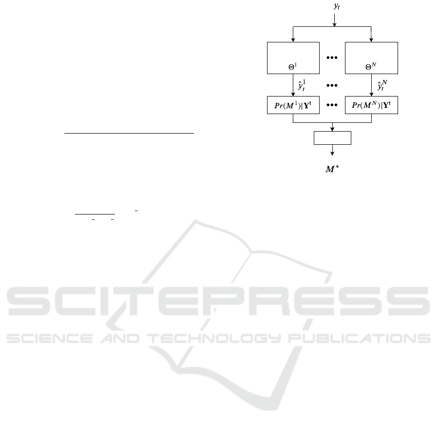
MAP

ExpertmodelN

Expertmodel1

Figure 1: AR-MM probabilistic framework with N expert

models acting as candidates to model the observed sequence

. The model M

∗

that has the highest posterior probability

is considered as the model that best represents the data.

Under this framework, N probabilities corre-

sponding to the N models are obtained at each time

instance with Equation (8). The model M

∗

that has

the maximum a posteriori (MAP) probability is then

considered as the model that best represents the in-

coming data from the set of available models. Figure

1 shows a block diagram of the AR-MM probabilistic

framework.

2.3 Standard SSVEP Detection

Methods

For the purpose of creating a reference against which

the new proposed method can be evaluated, a num-

ber of standard SSVEP detection techniques found in

the literature (Zerafa et al., 2018) were also imple-

mented. Similar to the proposed AR-MM probabilis-

tic framework, the following methods exploit only the

frequency information of the SSVEP signal, whereas

the phase information is not considered. The PSDA

method was chosen as a reference for the univari-

ate case since this is the simplest and most widely

used single-channel feature extraction method. For

the multivariate case, the CCA and FBCCA were se-

lected as reference methods. In the literature, the

CCA method is generally used as a reference method

against which new SSVEP methods are compared to,

while the FBCCA method, which is an extension of

CCA, has been shown to improve the frequency de-

tection of SSVEPs. A brief mathematical description

of these methods is presented below to better covey

the requirements of each technique and the frame-

work on which each is based.

An Autoregressive Multiple Model Probabilistic Framework for the Detection of SSVEPs in Brain-Computer Interfaces

2.3.1 Power Spectral Density Analysis (PSDA)

In PSDA a Fourier representation is used to transform

an EEG signal from the time domain to the frequency

domain and extract speciﬁc SSVEP features from the

resulting spectral content. The fast Fourier transform

(FFT) is performed on a single-channel EEG sig-

nal, from which the one-sided power spectral density

(PSD) (M

uller-Putz et al., 2008) is estimated. A fea-

ture vector is constructed from the PSD values at the

fundamental frequencies and harmonics correspond-

ing to the ﬂickering stimuli. A harmonic sum decision

(HSD) method (M

uller-Putz and Pfurtscheller, 2008)

is adopted to construct SSVEP feature vectors, where

the sum of harmonic power values for each stimulus

frequency f

is computed as:

∑

h=1

max

(PSD( f | f ∈ [h f

− 0.125,h f

+ 0.125])), (12)

where h represents the harmonic number being con-

sidered and H represents the number of harmonic fre-

quencies considered. The feature vector is log nor-

malised to make the features normally distributed.

The largest power amplitude is expected to corre-

spond to the frequency of the target stimulus, repre-

senting the SSVEP response.

2.3.2 Canonical Correlation Analysis (CCA)

CCA is a multivariable statistical method used to ﬁnd

the underlying correlation between two sets of data

(Lin et al., 2007), used to detect SSVEPs in multi-

channel EEG data. Let Y

Y and X

be two multidimen-

sional variables representing the multi-channel EEG

signals of length T samples and a set of SSVEP ref-

erence signals which have the same length as Y

Y , re-

spectively. The sine-cosine reference signals X

for

the target stimulus frequency f are deﬁned by:







sin(2πh f

)

cos(2πh f

)

sin(2πH f

)

cos(2πH f

)







t = 1,... ,T

h = 1,.. .,H

, (13)

where F

is the sampling frequency, T is the num-

ber of samples and H is the number of harmonics.

CCA ﬁnds the linear combinations y = Y

and

= X

, such that the correlation between the

two canonical variants y and x

is maximized (Lin

et al., 2007). The weight vectors W

and W

are

found by solving the following optimization problem

(Bin et al., 2009):

max

(y, x

) =

E[y

]

E[y

y]E[x

]

E[W

Y X

]

E[W

]E[W

]

(14)

For each reference signal, a maximum canonical cor-

relation ρ

is obtained and used as an SSVEP feature.

The hypothesis is that the reference signal with the

largest correlation contains SSVEP at the same fre-

quency as the stimulus signal.

2.3.3 Filter Bank Canonical Correlation

Analysis (FBCCA)

The FBCCA method is a CCA variant that decom-

poses SSVEPs into multiple sub-band components.

FBCCA performs separate CCAs between each of the

sub-band components and sine-cosine reference sig-

nals (Chen et al., 2015). The ﬁlter bank used consists

of sub-bands covering multiple harmonic frequency

bands. The correlation values between the sub-band

components Y

, k = 1,...,K from the original EEG

signals Y

Y and the reference signals X

correspond-

ing to all stimulation frequencies f are estimated to

form a correlation vector ρ

= [ρ

,..., ρ

]

, where

K is the number of sub-bands. A weighted sum of

squares of the correlation values corresponding to all

sub-band components is then calculated as the feature

for SSVEP detection as follows:

∑

k=1

w(k) · (ρ

)

, (15)

where w

w(k) are the weights of the sub-band compo-

nents. These weights are set by the observation that

the signal to noise ratio (SNR) of SSVEP harmonics

decreases as the response frequency increases:

w(k) = k

−a

+ b, k = 1,.. .,K , (16)

where a and b are constants that maximize the clas-

siﬁcation performance. The frequency of the refer-

ence signals having the maximum correlation is then

considered to be the target stimulus. The FBCCA

method requires three parameters to be optimized,

namely the number of harmonics to be considered in

the reference signals, the weight vector for the sub-

band components and the number of sub-bands in the

ﬁlter bank. Since these may interact with each other in

inﬂuencing the BCI performance (Chen et al., 2015;

Nakanishi et al., 2018), a grid search involving the si-

multaneous optimization of these parameters is con-

ducted using training data from various subjects. In

BIOSIGNALS 2020 - 13th International Conference on Bio-inspired Systems and Signal Processing

5 10 15 20 25 30 35 40 45 50

Frequency (Hz)

Amplitude

Figure 2: Spectra of the 12 AR models.

this work, based on the ﬁndings in the literature, the

number of harmonics, the weight vector, i.e. a and b

in Equation (16), and the number of sub-bands were

ﬁxed to 3, 1.25, 0.25 and 5, respectively.

3 RESULTS

In this section the application of AR models to

SSVEP data is ﬁrst described. Classiﬁcation results

of the AR-MM framework are then presented. This

is followed by a description of the training require-

ments of the probabilistic multiple model framework

and its classiﬁcation results compared to that of stan-

dard SSVEP detection methods.

3.1 AR Models Applied to SSVEP Data

The SSVEP data described in Section 2.1 consisted of

12 different classes, hence an AR model was trained

for each respective class. Training data was narrow

band pass ﬁltered around the ﬁrst H = 3 harmonic

frequency components corresponding to the actual

SSVEP response such that background activity not

corresponding to the SSVEP response is ﬁltered out

and hence not modelled. An AR model of order 20

was then ﬁt to the data. Given the narrow band ﬁlter-

ing done at the pre-processing stage, this model order

was found to give a good representation of the data ir-

respective of the stimulus class. A set of AR parame-

ters A

= {a

,...,a

}, for each model i = 1,..,N

was

then obtained using Burg’s method, where N

= 12

is the number of stimuli classes. Figure 2 shows the

spectra of 12 trained AR models, as an example.

When assigning a class to a new test trial y

, the

data is ﬁrst narrow band pass ﬁltered around the ﬁrst

three harmonic frequency components corresponding

to each of the 12 stimuli classes. Each trained AR

model, having AR parameter vectors x

, is then used

to estimate ˆy

, the predicted value of y

using Equation

(3). This process is shown in Figure 3.

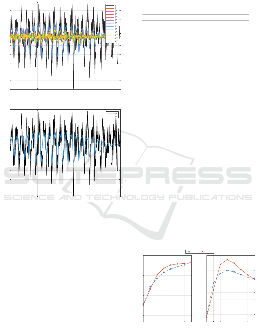
As an example, Figure 4a shows the original un-

ﬁltered signal and the narrow band pass ﬁltered sig-

nals estimated by each AR model for a 10.25 Hz test

trial. The errors between the original test signal y

and

the predicted signals ˆy

were estimated and the lowest

RMSE across the 2 s window was found. In this case

the minimum error was that between y

and ˆy

, shown

in Figure 4b. A difference between the two signals

can still be observed since the estimated signal is nar-

row band pass ﬁltered around the expected frequency

while the original signal is unﬁltered. Hence any ac-

tivity outside the bands of interest will not be mod-

elled. The correct model, however, is expected to best

represent the SSVEP related activity and hence result

in the smallest residual error. In the case being shown

here, this trial was correctly labelled as a class 7 trial,

corresponding to the 10.25 Hz SSVEP response.

3.2 Classiﬁcation Results of the

AR-MM Method

This section presents the classiﬁcation accuracy re-

sults when using the lowest RMSE of the 12 trained

models to classify each trial into one of the 12 avail-

able classes. The classiﬁcation accuracy was esti-

mated by considering only 1 trial per class as train-

ing data to generate the AR models, with the re-

maining 14 trials per class being used as testing data.

Cross validation was then carried out by repeating

the process such that each of the 15 trials was used

once for training purposes, and ﬁnally the average

classiﬁcation accuracy was computed. This analysis

was carried out on each bipolar channel combination

and the highest performance associated with the best

Filterfor

Figure 3: Process to ﬁnd residual errors between original

signal y

and estimated signals ˆy

for i = 1,..., 12 using 12

different AR models having parameter vectors x

to x

An Autoregressive Multiple Model Probabilistic Framework for the Detection of SSVEPs in Brain-Computer Interfaces

0 0.5 1 1.5 2

Time (s)

-12

-10

-8

-6

-4

-2

Amplitude

(a) Test data y

and estimated ˆy

in the time domain.

0 0.5 1 1.5 2

Time (s)

-12

-10

-8

-6

-4

-2

Amplitude

(b) Test data y

and estimated ˆy

in the time domain.

Figure 4: A 2 s SSVEP test trial at 10.25 Hz, represented

by class number 7 in the 12-class dataset.

bipolar channel (BBC) was found. The classiﬁcation

accuracy was also evaluated using different window

lengths for SSVEP detection. Apart from classiﬁca-

tion accuracy, the information transfer rate (ITR) in

bits per minute (bpm) (Wolpaw et al., 2002) was used

as a performance measure and was calculated as:

IT R =



log

+ Plog

P + (1 −P)log



1 − P

− 1



(17)

where P is the classiﬁcation accuracy, and T is the

average time for selection in seconds. An additional

gaze shifting time of 1 s was included in the estima-

tion of the ITR.

Figure 5 shows the average accuracy obtained

with the AR-MM framework, across all subjects and

sessions, for different data lengths ranging between

0.5 s to 4 s, in steps of 0.5 s. The proposed ap-

Table 1: AR-MM results for 12 classes (8.33 % chance clas-

siﬁcation accuracy) with 2 s window and 1 s gaze shift.

Subject Accuracy (%) ITR (bpm)

1 47.78 15.60

2 78.33 41.63

3 55.00 20.71

4 71.11 34.37

5 93.33 60.02

6 83.89 47.81

7 96.11 64.27

8 90.56 56.14

9 98.89 69.17

10 93.89 60.83

Mean ± STD 80.89 ± 16.88 47.05 ± 17.61

proach was compared to the PSDA method for which

the performance obtained with the BBC is also be-

ing reported for fair comparison. The PSDA re-

sults obtained are in line with those found in litera-

ture (Lin et al., 2007; Bin et al., 2009), although it

must be noted that direct comparison is difﬁcult due

to variations in BCI setups, such as the number of

stimuli being used. As expected, for both methods,

the SSVEP classiﬁcation increases with the length of

time window for detection. Paired t-tests were con-

ducted to analyse the difference in performance be-

tween the two methods across all the time windows.

These revealed that there is a statistically signiﬁcant

(p < 0.05) increase in performance for the AR-MM

method compared with the PSDA for time windows

between 1.5 s and 3 s.

To provide insight on individual subjects’ perfor-

mance, the results in Figure 5 for a time window of 2

s were expanded in Table 1.

This demonstrates that there is a large variation in

performance between subjects. In fact, the classiﬁca-

tion accuracy for 5 subjects is above 90%, for 3 sub-

jects this is between 70% and 90% and for 2 subjects

0.5 1 1.5 2 2.5 3 3.5 4

Time window (s)

100

Accuracy (%)

0.5 1 1.5 2 2.5 3 3.5 4

Time window (s)

ITR (bpm)

PSDA AR-MM

Figure 5: Performance comparison of PSDA and AR-MM

methods. (a) Average classiﬁcation accuracy (%) and (b)

ITR (bpm) across all subjects for different time windows

(s).

BIOSIGNALS 2020 - 13th International Conference on Bio-inspired Systems and Signal Processing

this is in the range of 50%.

These initial ﬁndings demonstrate that AR models

provide a good ﬁt for the SSVEP data and may be

used as a model structure in the multiple modelling

probabilistic framework.

3.3 Training for the Probabilistic

AR-MM Framework

Given the results obtained with the AR-MM approach

presented in the previous section, the AR multiple

models were incorporated within a probabilistic mul-

tiple modelling framework. The process of learning

the AR parameters x

and system parameters Θ

Θ in a

multiple modelling framework requires SSVEP train-

ing data for each class. Let z

be a vector of a sin-

gle channel SSVEP EEG data, with i = 1,...,N

rep-

resenting the number of target stimulus frequencies.

This data is then narrow band pass ﬁltered around

the fundamental frequency f and the ﬁrst H harmonic

components corresponding to the SSVEP class i and

is represented here by z

. The estimation of parame-

ters x

and Θ

Θ is then being carried out as follows:

• With reference to Section 3.1, the AR parameters

for the expert model M

are found using the ﬁl-

tered training data z

. AR parameters are esti-

mated using Burg’s method and the length of x

represents the AR model of order p which was

here set to 20.

• The unknown variance R is estimated from Equa-

tion (7), where the observation vector y

is re-

placed with training data z

, i.e. v

= z

− H

. In

this case H

represents p past narrow bandpass ﬁl-

tered training data, i.e. H

= [z

t−1

,...,z

t−p

]. The

variance σ

of the resulting v

is obtained from

each training trial of all the classes i = 1, ...,N

where l = 1, ...,L represents the number of train-

ing trials. The mean variance across all the train-

ing trials gives R, i.e. R = 1/(N

∑

i=1

∑

l=1

• The unknown covariance Q

for model M

is es-

timated from Equation (6), where for the non-

adaptive approach x

= Ix

+ w

. Therefore, the

covariance of x

∈ R

obtained from AR param-

eters across different training trials gives Q

∈

p×p

• As discussed earlier, following the non-adaptive

approach, the rest of the unknown system param-

eter are deﬁned as µ

µ = x

, Σ

Σ = Q

Q and Φ

Φ = I.

3.4 AR-MM Probabilistic Framework

In order to compare the performance of the AR-

MM probabilistic approach with that of the state-

of-the-art methods, batch mode classiﬁcation is con-

sidered in which each trial is ﬁrst segmented and

then passed through the AR-MM probabilistic pro-

cess. Labelling of one trial is done by ﬁnding

argmax

∑

t=1

Pr(M

), where N

is the total number

of samples in the time window.

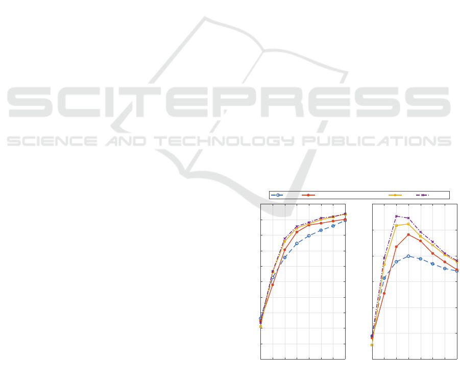
Figure 6 shows the average classiﬁcation accu-

racy and ITR obtained with the AR-MM probabilistic

framework across all subjects and sessions for differ-

ent data lengths from 0.5 s to 4 s, in steps of 0.5 s.

The classiﬁcation accuracy was estimated by con-

sidering 2 trials per class as training data to generate

the AR models x

, R and Q

Q and the remaining were

used for testing. A minimum of 2 training trials were

necessary to estimate the covariance Q

Q of the state

vector. This process was then repeated seven times

such that all trials were considered for training and an

average classiﬁcation accuracy was computed. The

performance of the AR-MM probabilistic approach is

compared with that of the PSDA, CCA and FBCCA

methods. In the case of both the AR-MM probabilis-

tic approach and the PSDA method, the performance

for each bipolar channel combination was computed

and the highest performance associated with the BBC

was found. On the other hand, all 8 channels were

used in the estimation of the CCA and FBCCA mul-

tivariate methods.

Two-way repeated measures ANOVA were per-

formed to compare the performance of the proposed

0.5 1 1.5 2 2.5 3 3.5 4

Time window (s)

100

Accuracy (%)

0.5 1 1.5 2 2.5 3 3.5 4

Time window (s)

ITR (bpm)

PSDA AR-MM probabilistic framework CCA FBCCA

Figure 6: Performance comparison of PSDA, AR-MM

probabilistic framework, CCA and FBCCA methods. (a)

Average classiﬁcation accuracy (%) and (b) ITR (bpm)

across all subjects for different time windows (s).

An Autoregressive Multiple Model Probabilistic Framework for the Detection of SSVEPs in Brain-Computer Interfaces

AR-MM probabilistic framework with each of the ref-

erence SSVEP detection methods across all the differ-

ent time windows. This indicated that there was a sta-

tistically signiﬁcantly (p < 0.05) improvement in the

overall SSVEP classiﬁcation accuracy with the AR-

MM probabilistic framework when compared with

the PSDA method. Post-hoc paired t-tests, which

considered the results from different time windows,

revealed that the AR-MM probabilistic method ob-

tained statistically signiﬁcantly (p < 0.05) higher ac-

curacies compared to PSDA method for time win-

dows 1.5 s - 3.5 s. The overall classiﬁcation accura-

cies of the multichannel methods, CCA and FBCCA,

were slightly higher than that of the single-channel

AR-MM probabilistic framework. In the case of the

FBCCA method, the accuracy was found to be sta-

tistically signiﬁcantly higher (p < 0.05) than the AR-

MM probabilistic approach for time windows of 1 s,

1.5 s and 4 s. These results indicate that the AR-

MM probabilistic approach can signiﬁcantly enhance

the performance of the single-channel PSDA method.

These results also show a slight decrease in perfor-

mance, speciﬁcally 2.29 % compared to the multi-

channel CCA method and 3.73 % compared to its

extension the FBCCA method on average over all

time windows, with the advantage of requiring only

a single-channel for SSVEP detection.

4 DISCUSSION

The results presented in Section 3 demonstrate that

the multiple model probabilistic framework is a

promising technique for the detection of SSVEPs in

BCIs.

Autoregressive models that capture the dynamics

of the underlying SSVEP signal in the EEG data were

used as a model structure for the AR-MM framework.

Initially an investigation was conducted to evaluate

whether AR models provide a good ﬁt for the data.

The standard approach of using AR models in EEG

analysis is to ﬁnd AR parameters for incoming EEG

data to form features which can then be used for clas-

siﬁcation (Guger et al., 2012; Saﬁ et al., 2018). In

this work however, AR expert models were trained

for each SSVEP class, each of which has a distinct

frequency, and then used for prediction on new EEG

data. The residual between the true and the recon-

structed signals was evaluated and used for classiﬁca-

tion. This was done since the MM framework is based

on the analysis of this residual which is speciﬁcally

used to calculate the likelihood function in Equation

(9). The initial classiﬁcation results of the AR-MM

framework using the RMSE as a basis for classiﬁca-

tion were compared to the PSDA method. The latter

is the simplest and one of the most commonly used

SSVEP detection methods, which similarly to the pro-

posed approach, operates on bipolar EEG channels.

It is worth pointing out that the classiﬁcation of the

PSDA method is done using features in the frequency

domain, speciﬁcally by analysing the power ampli-

tude of respective harmonics, while the classiﬁca-

tion of the AR-MM approach is done in the time do-

main, speciﬁcally by analysing the residual between

the original and the predicted signals. The results ob-

tained by the AR-MM approach showed a signiﬁcant

improvement in performance compared to the PSDA

method.

The second part of the analysis involved the re-

structuring of the AR-MM approach within a proba-

bilistic framework. In this case, a probability measure

for each model in representing incoming data was ob-

tained at each time instance and this result was then

evaluated to ﬁnd which model gave the best repre-

sentation within a ﬁxed time window, allowing batch

mode classiﬁcation as done with other state-of-the-art

techniques. In this case, apart from comparing the

performance of the AR-MM probabilistic framework

to a similar single bipolar channel PSDA method,

the framework was also compared to the multivariate

CCA and FBCCA methods. Similar to the proposed

AR-MM probabilistic framework, these methods ex-

ploit only the frequency information of the SSVEP

signal, whereas the phase information is not consid-

ered. This is particularly useful in BCI setups that

do not have phase coded stimuli. It must be high-

lighted that multichannel SSVEP detection methods

are known to beneﬁt from an optimized combination

of multiple signals. In fact it has been shown that this

results in a greater robustness against noise and hence

improved performance compared to single channel

methods (Friman et al., 2007; Bin et al., 2009). The

results obtained for the single-channel AR-MM prob-

abilistic framework showed signiﬁcant improvement

over the single-channel PSDA method but even more

promising, the results obtained were only slightly

lower compared to the multichannel methods for most

time windows of SSVEP detection. This means that

a BCI requires only a pair of electrodes to function

with the AR-MM probabilistic approach, making it

more practical for the user.

Various studies have shown that incorporating a

user’s training data signiﬁcantly improves the detec-

tion performance (Nakanishi et al., 2015). However,

the amount of training data signiﬁcantly varies be-

tween methods and this may result in long and tedious

training sessions (Zerafa et al., 2018). In this work it

was shown that the AR-MM probabilistic method re-

BIOSIGNALS 2020 - 13th International Conference on Bio-inspired Systems and Signal Processing

quires only 2 trials per class of training data to model

the AR models, hence only a few seconds of training

are actually required for a new BCI user. From a pre-

liminary analysis we have carried out, we identiﬁed

that increasing the number of training trials for the

AR-MM framework did not show statistical improve-

ments in performance. The transferability of train-

ing data in the AR-MM probabilistic approach from

one subject to another will also be addressed in future

work.

5 CONCLUSIONS

A novel autoregressive multiple model (AR-MM)

probabilistic framework for the detection of SSVEPs

for BCIs was presented in this paper. Through this

work we have shown that the univariate AR-MM

probabilistic approach can yield a signiﬁcant im-

provement in performance over PSDA, a standard

single-channel SSVEP detection method and is only

2.29 % and 3.73 % lower in classiﬁcation perfor-

mance compared to CCA and FBCCA, respectively,

two standard multichannel SSVEP detection meth-

ods. The proposed framework also provides a mea-

sure of probability for each SSVEP class, which can

be used as a measure of certainty in the decision mak-

ing process.

ACKNOWLEDGEMENTS

This work was partially supported by the project

BrainApp, ﬁnanced by the Malta Council for Science

& Technology through FUSION: The R&I Technol-

ogy Development Programme 2016.

REFERENCES

Babiloni, F., Cincotti, F., Babiloni, C., Carducci, F., Mat-

tia, D., Astolﬁ, L., Basilisco, A., Rossini, P. M., Ding,

L., Ni, Y., Cheng, J., Christine, K., Sweeney, J., and

He, B. (2005). Estimation of the cortical functional

connectivity with the multimodal integration of high-

resolution EEG and fMRI data by directed transfer

function. Neuroimage, 24(1):118–131.

Bin, G., Gao, X., Yan, Z., Hong, B., and Gao, S.

(2009). An online multi-channel SSVEP-based brain-

computer interface using a canonical correlation anal-

ysis method. J. Neural Eng., 6(4):046002.

Cerutti, S., Chiarenza, G., Liberati, D., Mascellani, P., and

Pavesi, G. (1988). A Parametric Method of Identiﬁca-

tion. IEEE Trans. Biomed. Eng., 35(9):701–711.

Chen, L. L., Madhavan, R., Rapoport, B. I., and Ander-

son, W. S. (2013). Real-time brain oscillation detec-

tion and phase-locked stimulation using autoregres-

sive spectral estimation and time-series forward pre-

diction. IEEE Trans. Biomed. Eng., 60(3):753–762.

Chen, X., Wang, Y., Gao, S., Jung, T.-P., and Gao,

X. (2015). Filter bank canonical correlation

analysis for implementing a high-speed SSVEP-

based brain–computer interface. J. Neural Eng.,

12(4):46008.

Fabri, S., Camilleri, K., and Cassar, T. (2011). Paramet-

ric Modelling of EEG Data for the Identiﬁcation of

Mental Tasks. In Biomed. Enigeering Trends Electron.

Commun. Softw., pages 367–386.

Fabri, S. G. and Kadirkamanathan, V. (2001). Functional

Adaptive Control : an Intelligent Systems Approach.

Springer London.

Friman, O., Volosyak, I., and Gr

aser, A. (2007). Mul-

tiple channel detection of steady-state visual evoked

potentials for brain-computer interfaces. IEEE Trans.

Biomed. Eng., 54(4):742–750.

Galka, A., Wong, K. K. F., and Ozaki, T. (2010). Modeling

Phase Transitions in the Brain. Model. Phase Transi-

tions Brain, pages 27–53.

Ghahramani, Z. (2001). An Introduction to Hidden Markov

Models and Bayesian Networks. J. Pattern Recognit.

Artif. Intell., 15(1):9–42.

Ghahramani, Z. and Hinton, G. E. (1998). Switching State-

Space Models. Dep. Comput. Sci. Univ. Toronto,

pages 1–28.

Guger, C., Allison, B. Z., Großwindhager, B., Pr

uckl, R.,

Hinterm

uller, C., Kapeller, C., Bruckner, M., Krausz,

G., and Edlinger, G. (2012). How many people could

use an SSVEP BCI? Front. Neurosci., 6(169):1–6.

Herrmann, C. S. (2001). Human EEG responses to 1-100

Hz ﬂicker: Resonance phenomena in visual cortex

and their potential correlation to cognitive phenom-

ena. Exp. Brain Res., 137(3-4):346–353.

Krusienski, D. J., McFarland, D. J., and Wolpaw, J. R.

(2006). An evaluation of autoregressive spectral es-

timation model order for brain-computer interface ap-

plications. Conf. Proc. IEEE Eng. Med. Biol. Soc.,

1:1323–6.

Liehr, S., Pawelzik, K., Kohlmorgen, J., and M

uller, K. R.

(1999). Hidden Markov mixtures of experts with an

application to EEG recordings from sleep. Theory

Biosci., 118(3-4):246–260.

Lin, Z., Zhang, C., Wu, W., and Gao, X. (2007). Frequency

recognition based on canonical correlation analysis

for SSVEP-Based BCIs. IEEE Trans. Biomed. Eng.,

54(6):1172–1176.

Miran, S., Akram, S., Sheikhattar, A., Simon, J. Z., Zhang,

T., and Babadi, B. (2018). Real-time tracking of se-

lective auditory attention from M/EEG: A Bayesian

ﬁltering approach. Front. Neurosci., 12(MAY):1–20.

uller-Putz, G. R., Eder, E., Wriessnegger, S. C., and

Pfurtscheller, G. (2008). Comparison of DFT and

lock-in ampliﬁer features and search for optimal elec-

trode positions in SSVEP-based BCI. J. Neurosci.

Methods, 168(1):174–181.

An Autoregressive Multiple Model Probabilistic Framework for the Detection of SSVEPs in Brain-Computer Interfaces

uller-Putz, G. R. and Pfurtscheller, G. (2008). Control

of an electrical prosthesis with an SSVEP-based BCI.

IEEE Trans. Biomed. Eng., 55(1):361–364.

Nakanishi, M. (2015). 12-class joint frequency-

phase modulated SSVEP dataset for

estimating online BCI performance

[https://github.com/mnakanishi/12JFPM SSVEP].

Nakanishi, M., Wang, Y., Chen, X., Wang, Y.-t., Gao,

X., and Jung, T.-p. (2018). Enhancing Detection of

SSVEPs for a High-Speed Brain Speller Using Task-

Related Component Analysis. IEEE Trans. Biomed.

Eng., 65(1):104–112.

Nakanishi, M., Wang, Y., Wang, Y.-t., and Jung, T.-p.

(2015). A comparison study of canonical correlation

analysis based methods for detecting steady-state vi-

sual evoked potentials. PLoS One, 10(10):e0140703.

Pardey, J., Roberts, S., and Tarassenko, L. (1996). A review

of parametric modelling techniques for EEG analysis.

Med. Eng. Phys., 18(1):2–11.

Regan, D. (1966). Some characteristics of average

steady-state and transient responses evoked by mod-

ulated light. Electroencephalogr. Clin. Neurophysiol.,

20(3):238–248.

Saﬁ, S. M. M., Pooyan, M., and Motie Nasrabadi, A.

(2018). SSVEP recognition by modeling brain activ-

ity using system identiﬁcation based on Box-Jenkins

model. Comput. Biol. Med., 101(August):82–89.

Samdin, S. B., Ting, C. M., Salleh, S. H., Ariff, A. K., and

Mohd Noor, A. B. (2013). Linear dynamic models

for classiﬁcation of single-trial EEG. Proc. Annu. Int.

Conf. IEEE Eng. Med. Biol. Soc. EMBS, (July):4827–

4830.

Stoica, P. and Moses, R. (2005). Spectral Analysis of Sig-

nals. Pearson Prentice Hall.

Vialatte, F. B., Maurice, M., Dauwels, J., and Cichocki, A.

(2010). Steady-state visually evoked potentials: Focus

on essential paradigms and future perspectives. Prog.

Neurobiol., 90(4):418–438.

Wang, Z., Xu, P., Liu, T., Tian, Y., Lei, X., and Yao,

D. (2014). Robust removal of ocular artifacts by

combining Independent Component Analysis and sys-

tem identiﬁcation. Biomed. Signal Process. Control,

10(1):250–259.

Wenchang, Z., Fuchun, S., Chuanqi, T., and Shaobo, L.

(2019). Linear Dynamical Systems Modeling for

EEG-Based Motor Imagery Brain-Computer Inter-

face. 1006(December 2018).

Wolpaw, J. R., Birbaumer, N., Mcfarland, D. J.,

Pfurtscheller, G., and Vaughan, T. M. (2002).

Brain–computer interfaces for communication and

control. Clin. Neurophysiol., 113:767–791.

Zerafa, R., Camilleri, T., Falzon, O., and Camilleri, K. P.

(2018). To train or not to train? A survey on training

of feature extraction methods for SSVEP-based BCIs.

J. Neural Eng., 15(051001).

Zhang, W., Sun, F., Tan, C., and Liu, S. (2016). Low-Rank

Linear Dynamical Systems for Motor Imagery EEG.

Comput. Intell. Neurosci., 2016.

Zhang, Y., Ji, X., and Zhang, Y. (2015). Classiﬁcation of

EEG signals based on AR model and approximate en-

tropy. Proc. Int. Jt. Conf. Neural Networks, 2015-

Septe.

BIOSIGNALS 2020 - 13th International Conference on Bio-inspired Systems and Signal Processing