Working Progress towards Lawn Mower Automation

Alfredo Ch

avez Plascencia

1 a

, V

ıt

ezslav Beran

1 b

, Jaroslav Rozman

1 c

and Aguilar Acosta Armando

2 d

BUT FIT IT4Innovations, Czech Republic

University of Guadalajara, School of Mechatronics,

Carretera Guadalajara - Ameca Km. 45.5, C.P. 46600, Ameca, Jalisco, Mexico

Keywords:

Mobile Robot, Nonlinear Control, Path Planning.

Abstract:

This paper is a working progress towards an automation of the Spider lawn mower (SLM) which is a four syn-

chronized steering wheel mobile robot. During the functioning, the SML must follow cutting grass edge with

no overlapping of a strip of cut grass and also satisfy slippage constrains. To this end, a small prototype called

Andromina which is a four-independent steering wheel mobile robot has been chosen to verify the control

approach. This paper proposes to implement a mathematical model that takes into account the kinematics and

dynamics of the mobile robot and also a nonlinear control strategy like the state feedback linearization. The

most important advantage of the proposed model-control strategy is that it takes into account the nonlinearities

of the system and a control law becomes a linear one. The path following tracking error has been veriﬁed by

the statistical approach called analysis t-test and also results of real data simulations have shown the effective-

ness of the proposed control strategy applied to a four-independent steering nonholonomic wheeled mobile

robot.

1 INTRODUCTION

Mobility and controllability of lawn mower ma-

chines (LMM) is still an immature open research ﬁeld

(Wasif, 2011). A brief review of the state of the art of

LMM is carried out in (Wasif, 2011) where it states

that (Smith et al., 2005) proposes a design of a mobile

robot which lacks to discuss propositions of mowing

operation. Moreover, static localization and dynamic

obstacle avoidance are overlooked. And, the system

is controlled manually lacking artiﬁcial intelligence.

(Bing-Min and Chun-Liang, 2008) suggests an opti-

mal route planning of a mobile robot where it does not

converge autonomously to the path. Moreover, obsta-

cle avoidance algorithm would work for static obsta-

cles not for dynamic ones. The fundamental idea of

LMM as a mobile robot is discussed in (Taj and Timo-

thy, 2008) lacking simulation and implementation re-

sults. The work done in (Wasif, 2011) suggests a mo-

tor schema architecture to control a LMM and also

the system suffers from slippage conditions. From

https://orcid.org/0000-0002-7505-5570

https://orcid.org/0000-0002-7495-6932

https://orcid.org/0000-0001-8443-433X

https://orcid.org/0000-0003-4920-527X

our point of view, the systems mentioned previously

lack a complete mathematical formulation of a LMM

that can potentially allow the system to be controlled

by some classical control strategies. They also lack

slippage uncertainties than can be added to the math-

ematical model of the system. The objective of this

proposal is to cope with some of the drawbacks pre-

sented in the previous works by adding a mathemati-

cal model and a control functionality to the system.

To this end, some control strategies for mobile

robots are found in the literature. For instance,

(Mathieu et al., 2017) uses a backstepping method

to address a four-wheel steering mobile robot fol-

lowing a path which an observer is used to esti-

mate the lateral sliding. (Krzysztof and Dariusz,

2004) also uses a backstepping approach to solve the

control issue and the stability is proof by the Lya-

punov technique. (Paulo and Urbano, 2005) shows

an input-output feedback-linearization method in dis-

crete mode for the path following of wheeled mobile

robots (WMRs) subject to nonholonomic constraints.

(Harwood, 2016) controls a automower 330x using

feedback linearization and with the feedback gain es-

timated using an LQ-controller.

The control strategy proposed in this article is

feedback linearization which is one of the most com-

Plascencia, A., Beran, V., Rozman, J. and Armando, A.

Working Progress towards Lawn Mower Automation.

DOI: 10.5220/0008924300990108

In Proceedings of the 17th International Conference on Informatics in Control, Automation and Robotics (ICINCO 2020), pages 99-108

ISBN: 978-989-758-442-8

mon approaches to control nonlinear systems. The

advantage of this technique is the transformation ion

of the nonlinear system into a linear one by means of a

proper transformation of variables. The intention is to

apply the control strategy to the SLM and due to the

Spider system is not available at the moment of this

work, the system Andromina has been taken into ac-

count to apply the model-control strategy. The Spider

(Spider, 2015) as well as the Andromina (Andromina,

2016b) mobile robots are shown in Figures 1 and 2

respectively.

2 METHODS

Robot operating system (ROS) (Quigley et al., 2009)

is suggested to be used to handle the automation of the

SLM. The navigation stack (NS) that comes with ROS

installation is a set of conﬁgurable nodes that need to

be set up properly to the dynamics of the mobile robot

in turn. In other words, the move base node is the

core of the navigation stack which offers interfaces

between sensors and algorithms for: localization, lo-

cal and global path planners, local and global maps.

For instance, the global map is formed by the gmap-

ping node, which is based on simultaneous localiza-

tion and mapping (SLAM). Then, during the work-

ing of the robot, the NS interacts with sensor read-

ings, localization, path planing and map algorithms to

avoid obstacles on the path in order to reach a speci-

ﬁed goal (Fox et al., 1999). Further on, the dynamic

window approach planner (DWAP) and the Dijkstra’s

algorithm nodes are used by the NS to guarantee ob-

stacle avoidance (Fox et al., 1997). Thus, given a

global path to follow the NS uses the costmap node

that takes in the sensor data to build and inﬂate a local

2D occupancy grid map. This package also provides

support to the DWAP that generates the velocity com-

mands that drive the robot from an initial to a ﬁnal

coordinate. In this approach, a nonlinear control node

has been created and inserted into the NS.

3 MATHEMATICAL MODEL AND

CONTROL

A four-independent steering wheeled mobile robot

model and nomenclature has been inspired from

(Ch

avez Plascencia and Dremstrup, 2011) and pre-

sented in Figure 3.

3.1 Kinematic Model

(Guy et al., 1996) imposes two restrictions to the kine-

matic model; a) Rolling without slipping and b) no

sidelong motion. Equations 1 and 2 are the restric-

tions to the wheels with respect to P

and, they can

also be arranged in a more compact form as shown in

Equations 3 and 4.

[cos(β

) sin(β

) l

sin(β

− α

)]R(θ)

ξ − r

= 0

(1)

[sin(β

) − cos(β

) − lcos(α

− β

)]R(θ)

ξ = 0

(2)

(β

)R(θ)

ξ − J

= 0 (3)

(β

)R(θ)

ξ = 0 (4)

where; i = 1,2,3,4, R(θ) is the 2D rota-

tion matrix from frame {E} to frame {W }, ξ =

,θ]

represents the robot pose at the point P

= [β

,β

]

is the steering wheel angle vector

and ψ

= [ψ

,ψ

]

is the rotation wheel angle

vector. (N.Sarkar and R.V.Kumar, 1992) deﬁnes q as

n generalized coordinates that fall into m restrictions

which can be organized as C(q, ˙q), where k represents

holonomic restrictions and m − k represents nonholo-

nomic restrictions as presented in Equation 5.

A(q) ˙q = 0 (5)

With

A(q) =



(β)R(θ) 0 −J

(β)R(θ) 0 0



(6)

˙q =



˙x

˙y



(7)

where; A(q) is a (m × n) full rank matrix.

Some remarks about C(q, ˙q) can be stated as fol-

lows:

• If a restriction equation is in the form C( ˙q) and

it can be integrated, such restriction is a holo-

nomic one.

• If a restriction equation is in the form C( ˙q) and

it can not be integrated, such restriction is a

nonholonomic one.

According to (Coelho and Nunes, 2003), the

Equation C

(q)S(q) = 0 can be obtained from Equa-

tion 5, where S(q) is a linear independent vector ﬁeld

and N(C) is the null space of C

(q). And, it is also

possible to deﬁne a velocity η(t) such that for all t,

then Equation 8 can be stated.

ICINCO 2020 - 17th International Conference on Informatics in Control, Automation and Robotics

100

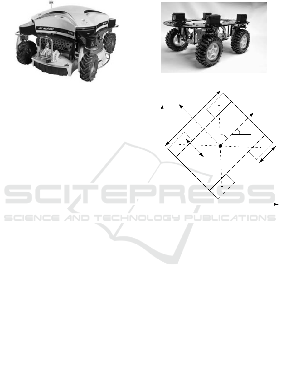
Figure 1: The Spider lawn mower robot.

˙q = S(q)η(t) (8)

Equation 8 gives a kinematic model.

In order to relate Equation 8 with the four-

independent steering wheeled kinematic model, the

no lateral movement constraint 4 is taken. It can be

seen that R(θ)

ξ lies in the null space of N (C

(β)).

Then, deﬁning N (C

(β)) = Σ(β) yields the follow-

ing relation N (C

(β))η(t) = Σ(t)η(t) = R(θ)

ξ. Af-

terwards, isolating

ξ from the previous equation and

then substituting it into Equation 3 and deﬁning the

steering velocity vector

β = ζ = [ζ

, ζ

], the

kinematic model is obtained as shown in Equation 9

which is of the form ˙q = S(q)u(t).



(θ)Σ(θ)



η(t)

(9)

According to (Guy et al., 1996), in order to guar-

antee maneuverability δ

of the SLM the degree of

mobility δ

and the degree of steeribility δ

, Equa-

tions 10 and 11 must satisfy the following conditions:

1 ≤ δ

≤ 3 and 0 ≤ δ

≤ 2.

= dimN [C

(β)] = 3 − rank[C

(β)] (10)

= rank[C

(β)] (11)

3.2 Dynamic Model

The relation between the torques τ derived by the em-

barked motors and the change in velocities ˙u in the

SLM can be described by the dynamic model. The

equations of motion that relates τ and ˙u can be de-

rived by means of the Lagrangian formalism as stated

in Equation 12, (Bloch, 2000; Symon, 1971; Gold-

stain, 1980).

∂L(q, ˙q)

∂ ˙q

−

∂L(q, ˙q)

∂q

= M

(q) ¨q +V (q, ˙q)

= A

(q)λ +B(q)τ (12)

Figure 2: Andromina.

f l

f r

{W }

{E}

Figure 3: The four-independent steering wheeled mobile

robot geometry. E is a ﬁxed frame on the robot with axis

and e

, W is world frame. θ is the angle of rotation, CM

is the center of mass.

The deﬁnition of the nomenclature in Equation 12 is

taken from (Ch

avez Plascencia and Dremstrup, 2011)

and stated as follows:

L(q, ˙q) is called the Lagrangian.

∈ R

n×n

is the matrix that represents the inertia

of the system.

V (q, ˙q) ∈ R

n×n

is the matrix of Coriolis.

A(q) is the matrix that represents the Jacobean.

B(q) ∈ R

n×(n−m)

is an input transformation ma-

trix.

τ ∈ R

(n−m)

is a torque vector that represents the

input.

λ ∈ R

is the Lagrangian multipliers.

q represents the generalized coordinates.

(Ch

avez Plascencia and Dremstrup, 2011) takes

the potential energy of the system as constant and it

is neglected from the Lagrangian multiplier. This fact

leads the Lagrangian L as function of the kinetic en-

ergy T, i.e. L = f (T ).

Working Progress towards Lawn Mower Automation

101

To solve Equation 12, the same methodology as

stated in (Ch

avez Plascencia and Dremstrup, 2011) is

applied. This is done in three steps. First, an individ-

ual kinetic energy of each wheel is solved. Second,

the kinetic energy of the chassis is also solved. And,

ﬁnally, all the energies are added to get a single en-

ergy.

The kinetic energy T

of a single steering wheel

attached to the trolley can be obtained by inte-

gration of an inﬁnitesimal mass d

[Kg] of a point

) which is placed on the surface of the

wheel. The radius r from the center of the wheel to

the point P

forms an angle ψ. Then, the velocity of

the point P

on the wheel is solved and then multi-

plied by the angular density ρ

[Kg/rad]. The former

process is shown in Equations 13 and 14.





+ lcos(α +θ) + rcos(ψ)cos(θ + β)

+ lsin(α +θ) + rcosψsin(θ+ β)

rsin(ψ)





(13)

2π

( ˙x

+ ˙y

+ ˙z

)ρ

dψ (14)

The kinetic energy of each individual wheel can

be obtained by inserting Equation 13 into Equation

14. The result is shown in Equation 15.

˙x

˙y

+ m

θ( ˙y

cos(α + θ)

− ˙x

sin(α + θ)) +

β +

(15)

= m

being the wheel’s inertia and m

2πρ

the mass’ wheel.

(Ch

avez Plascencia and Dremstrup, 2011) states

that the kinetic energy of a moving chassis can be ob-

tained by adding translational and rotational energies,

as it is presented in Equation 16.

( ˙x

+ ˙y

) +

(16)

˙x

= ˙x − d

θsin(θ + ρ) (17)

˙y

= ˙y + d

θcos(θ + ρ) (18)

Where; M

[Kg] is the chassis’s mass, ( ˙x

˙y

)[m/sec] is the linear velocity of the trolley about its

CM, I

[Kg · m

] is the inertia’s moment of the chassis,

θ[Rad/s] is the angular velocity and d[m] is the dis-

tance from the CM to the center of the robot.

Then, inserting 17 and 18 into 16, the Equation

19 is obtained. This equation represents the kinetic

energy of the chassis of the robot.

˙x

˙y

− M

d ˙x

θsin(θ + ρ) + M

d ˙y

θcos(θ + ρ)

(19)

By adding the individual wheel kinetic energy

with the chassis kinetic energy a total kinetic energy

is obtained as it can be seen in Equation 20.

T = T

∑

i=1

(20)

By expanding Equation 20 and then arranging it

into a matrix form gives Equation 21 which is the total

kinetic energy of the SLM with respect to its CM.

T =

R(θ)

MR(θ)

ξ +

W M

ψ +

θI

β (21)

W here :

W M







0 0 0

0 I

0 0

0 0 I

0 0 0 I











M =





0 M

0 0 M





= M

+ 4m

= −2

sin(ρ) + m

∑

i=1

sin(α

)

= 2

cos(ρ) + m

∑

i=1

cos(α

)

= d

+ I

+ m

∑

i=1

+ 2I

(22)

The dynamic model of the SLM with emphasis

in steering wheels can be derived according to the

procedure stated in (Guy et al., 1996). To this end,

the matrices A

(q) and B(q) = [0

3×8

8×8

] are re-

placed in the right expression of Equation 12. The

Lagrange equations of motion of the SLM with La-

grangian multipliers λ

and λ

are given by Equations

23 to 25.

ICINCO 2020 - 17th International Conference on Informatics in Control, Automation and Robotics

102



∂T

∂



−

∂T

∂ξ

=[T ]

= R

(θ)J

(β)λ

(θ)C

(β)λ

(23)



∂T

∂



−

∂T

∂β

=[T ]

=τ

(24)



∂T

∂



−

∂T

∂ψ

=[T ]

=−J

+ τ

(25)

The next step is to eliminate the Lagrange co-

efﬁcients from Equations 23 and 25. To do so,

the Equations 23 and 25 are premultiplied from the

left with Σ(β)R(θ) and Σ

(β)J

−T

respectively,

and then summed up and taking into account that

(β)C

(β) = 0

1×4

. This leads to two equations,

from which the Lagrange coefﬁcients have been dis-

appeared. Furthermore, the total kinetic energy Equa-

tion 21 is inserted in the left side of Equations 23,

24 and 25 respectively. Once [T ]

,[T ]

and [T ]

are

solved, they are inserted in the ﬁrst two equations

with no Lagrangian coefﬁcients. This step leads up

to two new equations that contain the velocity

ξ,

ψ,

β and acceleration

ξ,

ψ,

β terms. Then, with the aid

of the kinematic equations and their derivatives and

substituting them back and arranged them in a matrix

format yields the Equation 26 which is the dynamic

model of the system.

H(β) ˙u + f (β,u) = F(β)τ (26)

Where:

τ =





F(β) =



(β)E

(β) 0

4×4



P =





0 P

0 M





cos(θ) − M

sin(θ))

cos(θ) + M

sin(θ))

cos(θ) − M

sin(θ))

cos(θ) + M

sin(θ))

E(β) = J

−1

(β)

f (β,u) =



(β,u)



(27)

(β,u) = Σ

(β)

R(θ)

(θ) +R(θ)P

(θ)

−

R(θ)K

(β)N

(β)I

W M

E(β)

Σ(β)η

+Σ

(β)

R(θ)PR

(θ)

(β)I

W M

E(β)

Σ(β)η

(β,u) =

θI

H(β) =



(β) H

(β)

1×4

W M



(β) = Σ

(β)

R(θ)PR

(θ)

(β)I

W M

E(β)

Σ(β)

(β) =

(β)R(θ)K

The kinematics and dynamics of the SLM can be

written in state space representation as stated in Equa-

tions 28 and 29.

H(β) ˙u = − f (β,u) +F(β)τ (28)

˙q = S(q)u (29)

3.3 Control by Feedback Linearization

State feedback linearization has been chosen to tackle

the dynamics of the system. (Coelho and Nunes,

2003; Ch

avez Plascencia and Dremstrup, 2011) state

that if in a nonlinear system one or more restrictions

are nonholonomic the system is not fully state lin-

earizable, however it can be input-output linearizable.

One of the characteristics in input-output feedback

linearization is to ﬁnd a change of variables such that

z = T (x) and x = T

−1

(z) is diffeomorphism, bringing

the nonlinear system into a normal form. This form

decomposes the nonlinear system into external and in-

ternal parts respectively, making the system partially

linearizable. The output of the system in turn can see

the external variables but not the internal ones. The

external part can be linearized and be transformed into

a linear canonical form. It would be worth to analyz-

ing the stability of the internal part by means of the

zero dynamics of the system (Khalil, 2002; Marquez,

2003). When dealing with the external part, the num-

ber of output equations can be chosen by means of the

relative degree of the system.

Working Progress towards Lawn Mower Automation

103

To this end, the state representation stated in

Equations 28 and 29 is arranged in the following ma-

trix form.



˙q

˙u





S(q)u

−H

−1





−1



(30)

In the previous matrix expression, u is deﬁned as

[η,

]. Notwithstanding, the angular velocities

[

] are not taken into account because ˙q depends

only on η then u = η.

The state representation stated in Equation 30 can

be linearized by choosing a nonlinear feedback Equa-

tion τ = F

†

[Hν + f ] and it can also be arranged in a

general nonlinear form as shown in Equations 31, 32

and 33.

˙x = f (x)+ g(x)η

y = h(x) (31)



˙q





S(q)η







(32)

y = h(q)

˙x =



˙q



, f (x) =



S(q)η



, g(x) =





(33)

In order to achieve input-output linearization, an

analysis of the output equation y = h(q) must be

taken. In other words, the position vector q =

,θ] is of interest, then three output equations are

formulated as stated in the Equation 34.

h(q) =





(q)





= y =

















(34)

The output Equation 34 must be derived till it ﬁnds

the input

η (Khalil, 2002). Equation 35 shows that the

output y has been derived twice till it ﬁnds the input

η, thus having a relative degree ρ

= 2.

˙y

¨y

Jh(q)S(q)η

Φ(q)η + Φ

(35)

Where:

J =







∂q

∂x

∂q

∂y

∂q

∂θ







, Φ(q) = Jh(q)S(q)

(36)

J is the Jacobean. Since ˙q =

ξ = R

(θ)Σ(β)η

Equation 35 can also be arranged as follows:

˙y = R

(θ)Σ(β)η (37)

¨y =

(θ)Σ(β)η +R

(θ)

Σ(β)η + R

(θ)Σ(β)

A state variable transformation vector which is a

diffeomorphism as deﬁned in (Andersen et al., 2002)

is stated as follows.

z = T (q) =



1:6





1:3

, ˙y

1:3





˙y







h(q)

− − −

h(q)









h(q)

− − −

(θ)Σ(β)η





(38)

The system under the new state variable transfor-

mation vector T(q) is characterized by the following

dynamics:

˙z =



˙z

1:6





˙y

¨y





(θ)Σ(θ)η



z + B

β(z)[ν −α(z)]

(39)

Where:



3×3



, B



3×3



(40)

β(z) and α(z) are found by calculating



(θ)Σ(θ)η



as it is shown as follows:

β(z)[ν −α(z)] =



Σ(θ)η



W here :

β(z) = R

(θ)



Σ(β) S



α(z) = −β

−1

(z)

(θ)Σ(θ)η

ν =



η ζ







+ s

) (s

+ s

)

+ s

) (s

+ s

)

) (s

)





With :

= −l

cos(β

)sin(β

− α

)

= l

sin(β

)cos(β

− α

)

= −l

cos(β

)cos(β

− α

)

= l

cos(β

)sin(β

− α

)

= −l

sin(β

)cos(β

− α

)

= −l

cos(β

)cos(β

− α

)

= l

cos(β

)cos(β

− α

)

= l

sin(β

)sin(β

− α

)

= cos(β

− β

)

= −cos(β

− β

)

In the previous Equations ν = [

]

and

ν =

[

η ζ

]

, e.g. ν 6=

ν. This mean that the input to the

ICINCO 2020 - 17th International Conference on Informatics in Control, Automation and Robotics

104

Input

Reference

Linear System

˙z = A

z + B

of the

System

Output

−



ref



−K

Linear

Controller

+ +

z =



, ξ



˙z

Figure 4: Shows the linear system together with the refer-

ence input.

model ν given by equation 32 is not the same as the

input

ν given by the design control law. This problem

can be solved by differentiating the last two terms of

ν.

Moreover, the control law of the form

ν = α(z) +

−1

(z)ϑ transforms the system represented in Equa-

tion 39 into a linear one as it is shown in Equation

41.

˙z = A

z + B

ϑ (41)

This linearized system is a controllable one. And,

this can be easily veriﬁed by just looking at the ma-

trices A

and B

which are in controllable canonical

form. The vector ϑ which contains the accelerations

from the linear controller has to be designed in order

for the robot to follow a reference input r. Accord-

ing to the linear control theory (Franklin and Powell,

1994) the control input ϑ that allows the system to

follow the reference input r is stated in Equation 42.

ϑ = −Kz + (N

+ KN

) (42)

W here :

= −B

−1

= C

−1

r = [x

,θ, ˙x

, ˙y

θ]

Figure 4 shows the linearized system together with

the reference control input r.

4 CONTROL SIMULATION

RESULTS

The andromina ROAD-OFF V.2.0 robot (Andromina,

2016a) has been used as a test platform. It

has been equipped with the following hardware;

Lenovo ThinkPad L540 + Intel(R) Core(TM) i7-

4712MQ CPU @ 2.30GHz, Arduino Mega 2560

(Arduino, 2016), Four Micro DC motors with en-

coders (SKU, 2016), Four Servos, Hokuyo URG-

04LX-UG01 laser scanner (Hokuyo, 2009), Adafruit

Motor/Stepper/Servo Shield for Arduino v2 Kit -

v2.3 (Adafruit, 2016a), Adafruit 16-Channel 12-bit

PWM/Servo Shield (Adafruit, 2016b). Figures 5 and

6 show the Andromina and the implemented hard-

ware.

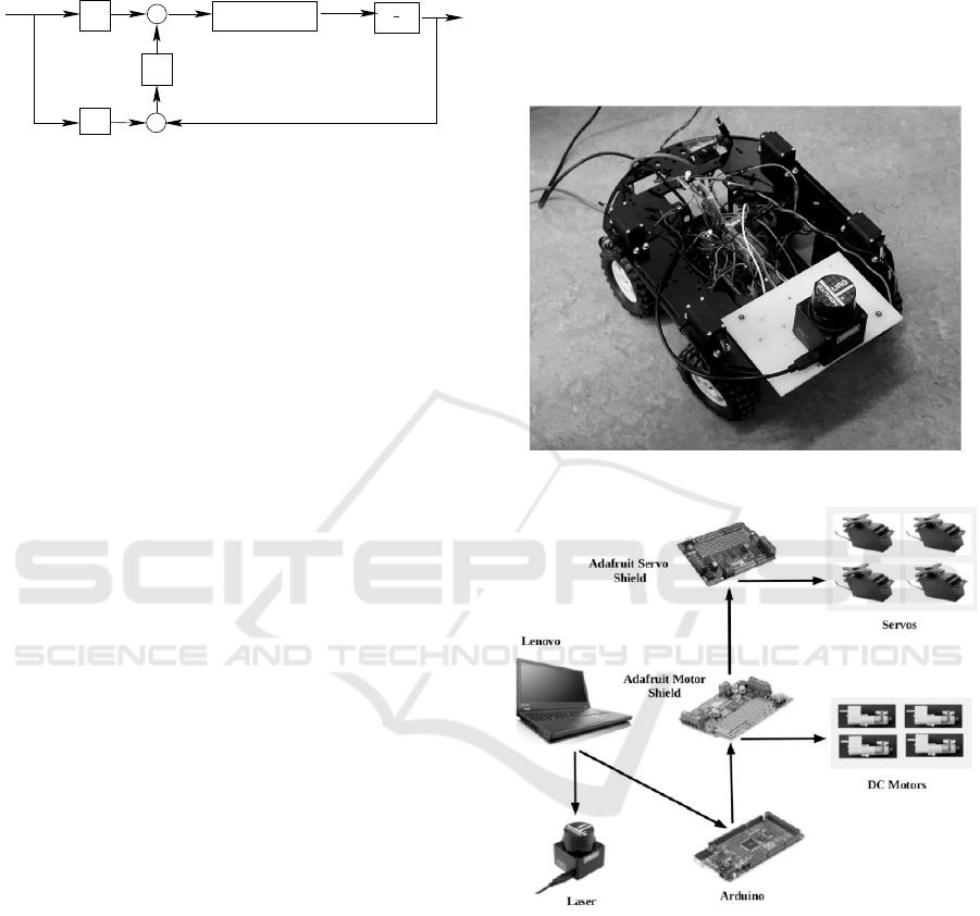
Figure 5: Shows the equipped andromina robot.

Figure 6: The Lenovo laptop communicates over a USB ca-

bles to the laser and Arduino. This in turn communicates

with the Adafruit motor and servo shields which communi-

cates with the four DC motors and four servos respectively.

The simulation has been carried out in two steps,

ﬁrstly it is simulated under Octave and secondly under

ROS.

4.1 Octave Simulation

A realistic path from a laboratory using a real map un-

der ROS-RVIZ have been taken and stored in memory

and then loaded with an Octave function for its anal-

Working Progress towards Lawn Mower Automation

105

(a)

(c)

(b)

(d)

Figure 7: (a) Angle β

. (b) Angle β

. (c) Angle θ. (d) Control trajectory and the reference input.

ysis. The results of the nonlinear control simulation

can be depicted in Figure 7(a-c). The angles β

and

are shown in Figure 7(a)(b). It can be seen that

these angles oscillate around 0 degrees, this means

that they do not move far from the robot chassis, in

other words, one can say that the nonlinear model

generates the proper steering angles for the wheels to

follow the trajectory path. Figure 7(c) depicts the an-

gle θ which is the angle of the robot chassis frame

with respect to the world frame. Finally, the ROS-

RVIZ planned trajectory is shown in Figure 7(d) as a

dark gray color whereas the nonlinear control that fol-

lows the planned trajectory is shown as a bright gray

color. It can easily be noticed how the control moves

the chassis [x

] according to the planned path and

as mentioned earlier.

The previous parameters β

, β

, θ and the nonlin-

ear control path tracking [x

] which are depicted

in Figure 7(a-c) have been taken as the inputs of an

Octave function called ”animation2(x

,θ,β

,β

)”.

The outcome of the simulated result is shown in Fig-

ure 8. In this ﬁgure, the position of the robot [x

]

is represented as an asterisk during the tracking path,

the chassis is represented as black square which cen-

ter is the position of the robot [x

], the wheels are

represented as black rectangles which center is placed

at each vertex of the chassis. It can be noticed that the

orientation of the wheels, angles β

, β

and β

correspond to the orientation of the tracking path and

the perpendicular wheel lines shall meet a single ICR.

-1 0 1 2 3 4 5

-0.4

-0.3

-0.2

-0.1

0.1

0.2

0.3

0.4

X [m]

Y [m]

[X, Y] position

Figure 8: Shows the chassis and position of the center of

gravity during the control trajectory. And, also shows the

position of the wheels according to the trajectory.

4.2 ROS Simulation

The results of the created ROS node that simulates

the nonlinear system can be depicted in Figures 9

and 10. At the start of the simulation, the ROS node

waits for the initial position which is achieved by left

mouse clicking on the ”2D Pose Estimate” RVIZ but-

ICINCO 2020 - 17th International Conference on Informatics in Control, Automation and Robotics

106

ton. Then, by left clicking on the ”2D Nav Goal”

RVIZ button a destination goal is chosen and the sta-

ble path is loaded and the control starts tracking the

reference path as it is depicted in Figure 10. It can

also be seen in this Figure that the laser position got

shifted.

Figure 9: The Figure shows the initial position and orienta-

tion of the robot.

Figure 10: The darkest line is the stable loaded path and the

less dark line is the tracking control. The shifted line is the

tracking laser position.

4.3 Independent t-test

By looking at the Figure 7(d) one can see that two tra-

jectories are almost identical, however it is necessary

to show if there is any statistical evidences to afﬁrm

or reject this statement. To this end, differences in the

two trajectories were assessed by t-test statistics. For

that, two hypothesis were established: null hypothesis

: µ

= µ

and alternative hypothesis H

: µ

6= µ

The aim of the t-test is to accept or reject the null hy-

pothesis. For that, two t-values are needed namely the

calculated t-value and the critical t-value. If the cal-

culated t-value is greater than the critical t-value then

the null hypothesis is rejected. In order to calculate

the t-value, the mean µ, variance σ

and sample size n

of each trajectory must be obtained. The t-value can

be computed by the Equation 43, whereas the criti-

cal t-value can be got from the t-table 1 which shows

that the calculated t-value is less than critical t-value.

Then, the null hypothesis can be accepted.

t =

− µ

(43)

Table 1: The table shows the mean, variance of the planned

trajectory as well as the control. It also shows the t-value

and the t-critical.

trajectory (n=60) Control (n=60)

Mean Variance Mean Variance

0.087 0.007 0.083 0.009

t-value 0.23585

t-critical 1.980

5 CONCLUSION

Nonlinear control is the strategy used to solve the

nonlinearities of the system. Moreover, the system

turned out to be a input output linearizable and with

a proper change of variables the system was trans-

formed into a linear one. Then, linear control strategy

was used for the path following. The Octave-ROS

simulated results have shown that the robot follows

the path and the steering angles are according to the

path trajectory. Furthermore, the two trajectories were

validated by the statistical t-test. In order to continue

with the progress of the automation of the Spider lawn

mower, the intention is to adapt the four independent

steering wheel Andromina model-control to the four

synchronized steering wheel Spider mobile robot. It

is necessary to research further under which condi-

tions the control is unstable or the control is robust. It

is also intended to compare the current control strat-

egy with other optimal control techniques, e.g. fuzzy

control, backstepping among others.

ACKNOWLEDGMENT

This work was supported by the project

IT4Innovations excellence in science, Czech

Ministry of Education, Youth and Sports LQ1602 and

by the project IGA FIT-S-20-6427.

REFERENCES

Adafruit (2016a). Adafruit Motor Shield. Available at https:

//www.adafruit.com/product/1438.

Working Progress towards Lawn Mower Automation

107

Adafruit (2016b). Adafruit Servo Shield. Available at https:

//www.adafruit.com/product/1411.

Andersen, P., Pedersen, S. T., and Dimon, J. (2002). Ro-

bust feedback linearization-based control design for a

wheeled mobile robot. Proc. of the 6th Interna- tional

Symposium on Advanced Vehicle Control.

Andromina (2016a). Andromia OFF-ROAD. Available at

http://androminarobot.blogspot.mx/ p/montaje.html.

Andromina (2016b). Andromina v.1.2. Available at http:

//androminarobot.blogspot.cz/ search/label/ Arduino.

Arduino (2016). Arduino Mega 2560. Available at https:

//www.arduino.cc/ en/ Main/arduinoBoardMega2560.

Bing-Min, S. and Chun-Liang, L. (2008). Design of an au-

tonomous lawn mower with optimal route planning. In

Industrial Technology, 2008. ICIT 2008. IEEE Inter-

national Conference on, pages 1–6, Chengdu. IEEE.

ISBN: 978-1-4244-1705-6.

Bloch, A. M. (2000). Nonholonomic Mechanics and Con-

trol. Addison-Wesley Publishing Company. ISBN:

0-387-95535-6.

avez Plascencia, A. and Dremstrup, K. (2011). Differen-

tial mobile robot based wheelchair. Technical report,

Aalborg University.

Coelho, P. and Nunes, U. N. (2003). Lie algebra application

to mobile robot control: a tutorial. Robotica, 21:483–

493.

Fox, D., Burgard, W., Frank, D., and Thrun, S. (1999).

Monte carlo localization: Efﬁcient position estimation

for mobile robots. In in proc. of the national confer-

ence on artiﬁcial intelligence, AAAI, pages 343–349.

Fox, D., Burgard, W., and Thrun, S. (1997). The dynamic

window approach to collision avoidance. Robotics &

Automation Magazine, IEEE, 4(1):23–33.

Franklin, G. F. and Powell, J. D. (1994). Feedback Control

of Dynamic Systems, third edition. Addison-Wesley.

ISBN: 0-201-53487-8.

Goldstain, H. (1980). Nonholonomic Mechanics and Con-

trol. Addison-Wesley. ISBN: 0-201-02918-9.

Guy, C., Georges, B., and Brigitte, D. A.-n. (1996). Struc-

tural properties and classiﬁcation of kinematic and dy-

namic models of wheeled mobile robots. IEEE Trans-

actions on Robotics and Automation, pages 47–62.

Harwood, P. (2016). Non-linear automatic control of au-

tonomous lawn mower. Master’s thesis, Link

oping

University, SE-581 83 Linkoping, Sweden.

Hokuyo (2009). URG-04LX-UG01. Available at

https://www.hokuyo-aut.jp/02sensor/ 07scanner/

urg 04lx ug01.html.

Khalil, H. (2002). Nonlinear Systems. Prentice Hall. ISBN:

0-13-067389-7.

Krzysztof, K. and Dariusz, P. (2004). Modeling and con-

trol of a 4-wheel skid-steering mobile robot. Interna-

tional Journal of Applied Mathematics Computer Sci-

ence, 14(4):477–496.

Marquez, H. J. (2003). Nonholonomic Control Systems

Analysis and Design. Wiley. ISBN: 0-471-42799-3.

Mathieu, D., Roland, L., Adrian, C., Christophe, C., and

Benoit, T. (2017). Path tracking of a four-wheel steer-

ing mobile robot: A robust off-road parallel steer-

ing strategy. IEEE European Conference on Mobile

Robots (ECMR).

N.Sarkar, N. and R.V.Kumar (1992). Control of mechanical

systems with rolling constraints: Application to dy-

namic control of mobile robots. Technical report, De-

partment of Computer & Information Science (CIS),

University of Pensylvania.

Paulo, C. and Urbano, N. (2005). Path-following control

of mobile robots in presence of uncertainties. IEEE

International Journal of Transactions on Robotics,

21(2):452–261.

Quigley, M., Conley, K., Gerkey, B., Faust, J., Foote, T. B.,

Leibs, J., Wheeler, R., and Ng, A. Y. (2009). ROS: an

open-source robot operating system. In ICRA Work-

shop on Open Source Software.

SKU (2016). DC Motor with Encoder. Avail-

able at https:// www.dfrobot.com/wiki/ index.

php/Micro DC Motor with Encoder-SJ02 SKU:

FIT0450.

Smith, J., Campbell, S., and Morton, J. (2005). Design

and implementation of a control algorithm for an au-

tonomous lawnmower. In Circuits and Systems, 2005.

48th Midwest Symposium on, volume 1, pages 456–

459, Covington, KY. IEEE. ISBN: 0-7803-9197-7.

Spider (2015). Mini, ILD01, ILD02. Available at https:

//www.slope-mower.com/ spider-ild01 p12.html.

Symon, K. R. (1971). Mechanics. Addison-Wesley World

student series. Addison-Wesley Publishing Company.

ISBN: 9780201073928.

Taj, B. M. and Timothy, K. T. C. (2008). Design and mod-

elling a prototype of a robotic lawn mower. In Infor-

mation Technology, 2008. ITSim 2008. International

Symposium on, volume 4, pages 1–5, Kuala Lumpur,

Malaysia. IEEE. ISBN: 978-1-4244-2327-9.

Wasif, M. (2011). Design and implementation of au-

tonomous lawn-mower robot controller. In 7th In-

ternational Conference on Emerging Technologies

(ICET), pages 1–5. IEEE. ISBN: 978-1-4577-0769-

ICINCO 2020 - 17th International Conference on Informatics in Control, Automation and Robotics

108