Optimal Pipe Routing Techniques in an Obstacle-Free 3D Space
Marvin Stanczak
1,2
, C
´
edric Pralet
1
, Vincent Vidal
1
and Vincent Baudoui
2
1
ONERA/DTIS, Universit
´
e de Toulouse, F-31055 Toulouse, France
2
Airbus Defence and Space, Toulouse, France
Keywords:
Pipe Routing, Automation, Optimization, Constraints.
Abstract:
This paper introduces two approaches to automate the design of pipe-systems in a continuous 3D space to
assist designers to deal with the high number of constraints of the pipe routing problem. This work assimilates
a pipe to a succession of straight sections and bends in which possible bends are restricted to a bend catalog
containing orthogonal and non orthogonal bends. As a preliminary work, both methods ignore obstacles but
take into account pipe section orientations to deal with asymmetrical pipe sections. To do so, a graph of
reachable pipe orientations is generated from the bend catalog. Then, the first approach enumerates valid
bend combinations using the previous graph and computes the optimal length of straight sections for each
combination using a Linear Program. The second one formulates the pipe routing problem as a Mixed Integer
Linear Programming problem based on enumerated reachable orientations. Both approaches are tested on
realistic scenarios inspired by industrial problems.
1 INTRODUCTION
For some industries, the design of piping-systems
plays an important role because of the large number
of pipes to be routed, like in aircraft or spacecraft de-
sign, shipbuilding, circuit layout or plant layout. It
is an highly time-consuming phase in industry. Tra-
ditionally, pipe designers manually define routes and
have to deal with a lot of constraints. For these rea-
sons, many researches have been conducted to auto-
mate the pipe routing process in order to save time
and money during the design phase.
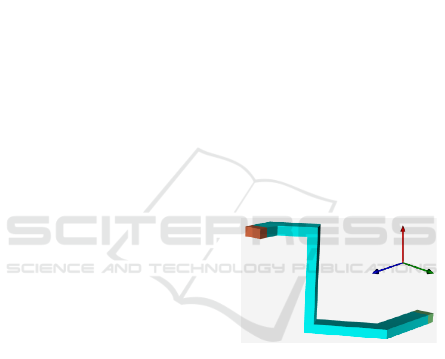
In practice, pipe designers build a route as a
succession of rigid straight sections and rigid bends
using their expertise to choose the best routing spaces
and save length and bends (see Figure 1). The differ-
ent bends they can use are defined by catalogs from
pipe manufacturers. Various kinds of bends are often
available, not just orthogonal ones (a bend is said to
be orthogonal when the direction of the pipe before
the bend is orthogonal to the direction of the pipe
after the bend). Historically, the classic pipe routing
algorithm, called ”Maze algorithm”, was introduced
by Lee (Lee, 1961). In this approach, the routing
environment is discretized with a regular grid and the
cells which are occupied by obstacles are labeled.
Then, starting from the source cell, the best route is
Figure 1: Example of a routed pipe.
computed by exploring the cells’ neighborhood un-
til the target is reached. This kind of cell decom-
position approach was improved using different al-
gorithms which require less memory space like Ant
Colony Optimization (Fan et al., 2006; Jiang et al.,
2015), Genetic Algorithm (Ito, 1999; Kimura, 2011)
or Particle Swarm Optimization (Asmara and Nien-
huis, 2006). Recently, Belov also introduced a Con-
straint Programming formulation (Belov et al., 2017).
However, cell decomposition is not adapted to non or-
thogonal bends, even if Ando proposed to introduce
additional edges in the cell adjacency graph to model
complex bends (Ando and Kimura, 2012). It is also
possible to build pipes by adding elements one by one
from a catalog containing bends and straight sections
Stanczak, M., Pralet, C., Vidal, V. and Baudoui, V.
Optimal Pipe Routing Techniques in an Obstacle-Free 3D Space.
DOI: 10.5220/0008923300690079
In Proceedings of the 9th International Conference on Operations Research and Enterprise Systems (ICORES 2020), pages 69-79
ISBN: 978-989-758-396-4; ISSN: 2184-4372
Copyright
c
2022 by SCITEPRESS – Science and Technology Publications, Lda. All rights reserved
69

(Furuholmen et al., 2010), but this approach does not
guarantee to find a feasible solution even if there ex-
ists one in a continuous space. Indeed, some points
of the space are unreachable from a given catalog of
pipe elements.
Other methods, called Skeleton approaches, build
a graph of possible route candidates using rules in-
spired by experience. This way, the pipe routing prob-
lem can be modeled as a shortest path problem in
a graph, solved using the Dikjstra algorithm (S.-H.
et al., 2013) or Mixed Linear Integer Programming
(Guirardello and Swaney, 2005). A more recent re-
search also explored Evolutionary Algorithms consid-
ering multi-objective routing in a skeleton graph (Liu
and Liu, 2018).
While cell decomposition approaches discretize
the environment and the pipes, skeleton-based algo-
rithms reduce the possible solutions to a finite set. In
both cases, these methods lead to sub-optimal solu-
tions in the continuous space. To improve the quality
of the solutions, Zhu uses cell decomposition to de-
fine a routing channel and then computes the detailed
route using a projection procedure (Zhu and Latombe,
1991). Park proposes a method that generates routing
cells adapted to the environment and uses patterns in-
side these cells (Park and Storch, 2002).
Another way to build a route in a continuous en-
vironment is to extend lines from the origin point us-
ing a set of directions and repeat this extension each
time a line intersects an obstacle until the destination
is reached. This approach, called ”Escape Algorithm”
or ”Line Search Algorithm”, was introduced by High-
tower (Hightower, 1969) and allows to deal with non
orthogonal bends. But such methods do not take into
account the orientation of the pipe sections. Indeed,
some types of pipes can have centerline unsymmetri-
cal sections such as rectangular sections. In this case
the route must reach the destination with the right
orientation, that is with the right angular position of
the section around the centerline. This is not possi-
ble with line search methods which only consider the
centerline.
Last, some parametric-based models were also
proposed using adaptable pipe patterns. In this case,
the pipe route can be optimized using Mathematical
Programming (Sakti et al., 2016; Medjdoub and Bi,
2018) or Genetic Algorithms (Ikehira et al., 2005).
However, existing models do not consider bend cata-
logs with non orthogonal bends.
This paper introduces two pipe routing algorithms
which respond to the following three challenges:
• ensure solution optimality in a 3D continuous
routing space; optimality is evaluated here with
regards to the total cost of the pipe, given by the
sum of the costs of each individual bend and each
individual straight section used (more details later
on these points),
• use non orthogonal bends from a catalog,
• take into account unsymmetrical pipe sections.
For this purpose, as a first necessary step for future
works, a simplified version of the Pipe Routing Prob-
lem in 3D space (3D-PRP) is considered: the 3D
Obstacle-Free Pipe Routing Problem (3D-OFPRP) in
which no obstacles are taken into account. Note that
in the obstacle-free problem, we consider both that
there is no external obstacle and that the pipe cannot
be an obstacle for itself. The relaxation of these two
assumptions are left for future works.
The first proposed approach, presented in Section
3, decomposes the problem into a shortest path prob-
lem in an oriented graph and a Linear Programming
(LP) problem. The second one, presented in Section
4, is based on a Mixed Integer Linear Programming
(MILP) model. Both approaches require geometric
notations introduced in Section 2 to make the linear
formulations possible. Section 5 describes experi-
mental results for both methods. Last, Section 6 gives
perspectives on the way obstacles can be taken into
account.
2 PROBLEM DEFINITION
2.1 Geometric Preliminaries
In what follows, a pipe is described as a succession
of straight sections and bends. This representation is
formalized in this section.
2.1.1 Local Pipe Configurations
We consider a 3D Cartesian coordinates system de-
fined by its origin point and its standard orthonormal
basis (
−→
e
x
,
−→
e
y
,
−→
e
z
) where
−→
e
x
= (1,0,0),
−→
e
y
= (0,1,0),
and
−→
e
z
= (0, 0,1). In this system, the vector of coor-
dinates of a point P are referred to as
−→
p = (P
x
,P
y
,P
z
)
and the coordinates of a vector are referred to as
−→
v = (v
x
,v
y
,v
z
).
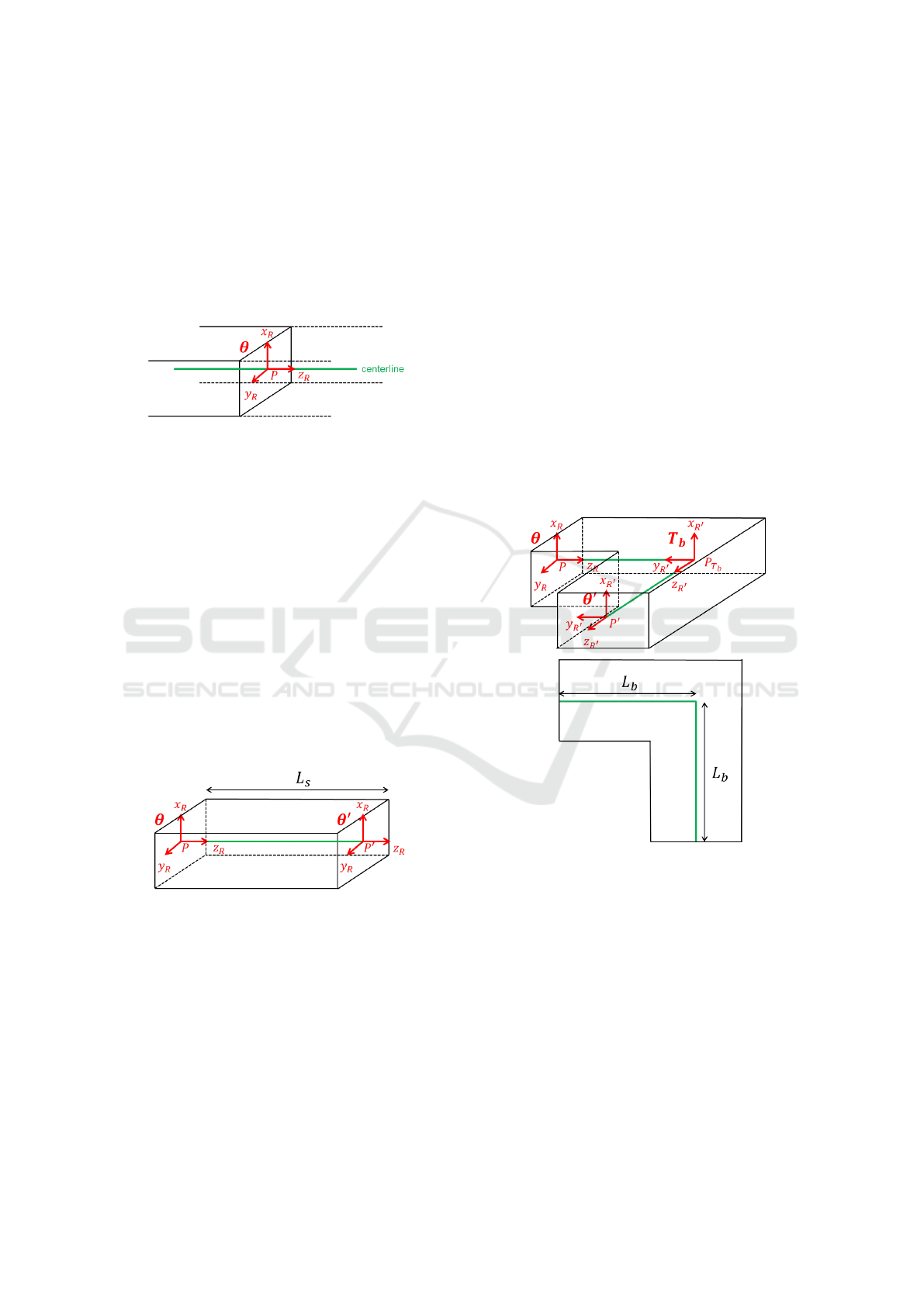
For a pipe with any section and any point P of the
centerline of the pipe, it is possible to define the local
configuration of the pipe at point P as the pair θ =
(P,R) where R is an orthonormal basis (
−→
x
R
,
−→
y
R
,
−→
z
R
)
such that (1) vector
−→
z
R
is collinear with the center-
line and (2) the intersection between the volume of
the pipe and plane (P,
−→
x
R
,
−→
y
R
) matches exactly with
the section of the pipe (see Figure 2). Equivalently,
R corresponds to a rotation matrix which defines how
ICORES 2020 - 9th International Conference on Operations Research and Enterprise Systems
70
to transform the orthonormal basis of the 3D coor-
dinates system into the orthonormal basis associated
with the local configuration.
In the following, R is called the orientation of lo-
cal configuration θ and the set of pipes’ local configu-
rations is referred to as Θ. Note that we consider here
that there is a unique shape for the pipe section all
along the pipe (for example, not possible to transform
a square pipe section into a rectangular pipe section).
Figure 2: A local pipe configuration.
For any part of a pipe, the input configuration (re-
spectively the output configuration) is the local con-
figuration associated with the first end section (re-
spectively the last end section) of the pipe part.
2.1.2 Straight Sections
With the previous notations, the output configuration
of a straight section of a pipe of length L
s
∈ R
+
ap-
plied from the local configuration θ = (P, R) ∈ Θ is the
local configuration θ
0
= (P
0
,R) where P
0
is the point P
translated of the distance L
s
along vector
−→
z
R
(see Fig-
ure 3). Thus, a straight section can be represented by
an application s from Θ into Θ defined by a length L
s
.
S refers to the set of straight sections of pipes. The
cost C
s
of a straight section s ∈ S is αL
s
where α is a
constant linear cost.
Figure 3: A straight section.
2.1.3 Bends
As for straight sections, the output configuration of a
bend of rotation matrix R
b
and half length L
b
∈ R
+
applied from the local configuration θ = (P, R) ∈ Θ is
the local configuration θ
0
= (P
0
,R
0
) where R
0
= RR
b
and P
0
is the point P translated of the distance L
b
along vector
−→
z
R
and then translated of the distance L
b
along vector
−→
z
R
0
(see Figure 4). Rotation matrix R
b
expresses the orientation of the output configuration
of the bend in the basis associated with its input con-
figuration.
Thus, a bend can be represented by an application
b from Θ into Θ defined by a rotation matrix R
b
and a
half length L
b
. By extension, a bend b also transforms
an input orientation o into an output orientation o
0
re-
ferred to as o
0
= b(o). In the following, B refers to the
set of bends. The definitions provided are also valid
for bends leading to a twisted pipe section between
two straight sections.
The cost of a bend b ∈ B is referred to as C
b
∈ R
+
.
For each bend b ∈ B applied from configuration
θ = (P, R) ∈ Θ, the transition configuration is the lo-
cal configuration of the pipe T
b
=
P
T
b
,R
T
b
where
R
T
b
= RR
b
and P
T
b
is the point P translated of the
distance L
b
along vector
−→
z
R
(see Figure 4). In other
words, the transition configuration of bend b is the
local configuration with the break point of the center-
line as origin and the output orientation of the bend as
orientation.
Figure 4: A bend b and its transition configuration T
b
.
Note that in practice, a bend is not a discontinu-
ous change of the centerline direction. The center-
line follows a circular arc depending on the angle of
the bend and on the bend radius. But the introduced
representation guarantees that, between two transition
configurations, the centerline section is a segment of
R
3
, which is used in what follows.
2.1.4 Bend Combinations
A bend combination B is a list [b
1
,..., b
N
B
] of
bends in B. N
B
refers to the number of bends of com-
bination B. By extension, B also transforms an input
Optimal Pipe Routing Techniques in an Obstacle-Free 3D Space
71

orientation o into an output orientation B(o) defined
by:
B(o) = b
N
B
◦ ... ◦ b
1
(o) (1)
The cost of a bend combination B is defined by:
C
B
=
N
B
∑
i=1
C
b
i
(2)
2.1.5 Pipes
With the previous notations, a pipe Π with
N
Π
∈ N bends can be described by a list
[s
1
,b
1
,s
2
,..., s
N
Π
,b
N
Π
,s
N
Π
+1
] alternating N
Π
+ 1
straight sections s
i
∈ S and N
Π
bends b
i
∈ B. Thus,
any pipe can be represented by an application Π from
Θ into Θ that verifies the following conditions:
Π (θ) = s
N
Π
+1
◦ b
N
Π
◦ s
N
Π
◦ ... ◦ s
2
◦ b
1
◦ s
1
(θ) (3)
P refers to the set of pipes. For N ∈ N, P (N)
refers to the set of pipes which contain exactly N
bends and P
max
(N) refers to the set of pipes which
contain at most N bends.
The cost C
Π
∈ R
+
of such a pipe is defined by the
cost of its bends and straight sections:
C
Π
=
N
Π
∑
i=1
C
b
i
+
N
Π
+1
∑
i=1
αL
s
i
(4)
If the input configuration θ and the output config-
uration Π (θ) of a pipe Π ∈ P are considered as tran-
sition points, the centerline of Π can be described as
a sequence of transition configurations:
Π = [T
0
,..., T
N
Π
+1
] (5)
with
T
0
= θ,
T
N
Π
+1
= Π (θ),
and ∀i ∈
{
1,..., N
Π
}
, T
i
= T
b
i
2.2 Constraints
The 3D-OFPRP can be subject to various kinds of
constraints depending on the application field (Park
and Storch, 2002). This section enumerates the con-
straints taken into account in our study.
2.2.1 Routing Space
A pipe should be routed within a finite subset A of
R
3
called the routing space. In what follows, it is as-
sumed that A is a convex subset of R
3
described by a
set of inequalities:
∀i ∈
{
1,..., k
A
}
A
i
x + B
i
y +C
i
z + D
i
≤ 0 (6)
So, because of the convexity of A, the centerline
of the pipe Π ∈ P is contained in the routing space if
and only if all the transition configurations of Π are in
the routing space.
2.2.2 Catalog of Bends
Pipe designers can be led to use a restricted set of
bends in order to reduce production costs. This set of
possible bends is referred to as B
cat
⊆ B . It contains
N
B
cat
bends.
2.2.3 Pipe Attachability Constraints
In practice, the way pipes are routed is subject to
physical constraints. For instance, pipes are supported
by brackets which are fitted to fixed planar structures
referred to as walls. W is the set of walls. A pipe
configuration θ = (P,R) ∈ Θ is attachable to a wall
w ∈ W of normal
−→
n
w
if and only if:
−→
x
R
·
−→
n
w
= 0 ∨
−→
y
R
·
−→
n
w
= 0 (7)
This means that, for a pipe whose section is rectan-
gular, at least one edge of the section is parallel to
wall w. This way, a bracket can be used to fix the
pipe at the point corresponding to pipe configuration
θ = (P, R). Also, the actual distance between the pipe
and the wall to which it is attached can be limited just
by restricting the routing space.
By extension, a pipe Π ∈ P is attachable to W
if and only if all the transition configurations of Π
are attachable to at least one wall w ∈ W . So, as a
pipe configuration constraint, the routed pipe should
be attachable to W .
2.2.4 Minimal Length of Straight Sections
In order to respect the pipe manufacturing constraints,
each straight section of a pipe Π ∈ P must have a min-
imal length L
min
.
2.3 Goal
For a maximum number of bends N
max
∈ N, the 3D-
OFPRP consists in connecting a source configura-
tion θ
s
= (P
s
,R
s
) ∈ Θ to a destination configuration
θ
d
= (P
d
,R
d
) ∈ Θ using a pipe Π ∈ P
max
(N
max
) min-
imizing the pipe cost C
Π
and respecting the previous
constraints.
Furthermore, for n ∈
{
0,..., N
max
}
, the 3D-
OFPRP(n) consists in the same problem but with
pipes Π ∈ P (n) containing exactly n bends. This way,
the optimal solution of the 3D-OFPRP is the best so-
lution among the optimal solutions of the set of 3D-
OFPRP(n) for n from 0 to N
max
.
ICORES 2020 - 9th International Conference on Operations Research and Enterprise Systems
72
3 COMBINED GRAPH-LP
SOLVER
This section introduces a formulation of the 3D-
OFPRP which uses a graph structure representing all
pipe orientations that can be reached from the source
orientation with at most N
max
bends of catalog B
cat
.
3.1 Preprocessing: Reachable
Orientation Graph
To enumerate the reachable orientations, an oriented
graph G (O,E) is built iteratively using the reachable
orientations as vertices and the bends that allow to
reach an orientation from another one as arcs.
The generation procedure of the graph starts by
adding the source orientation R
s
to G (O, E). Then,
the graph is extended by applying each bend b of cata-
log B
cat
to each node o ∈ O added at the previous step.
If the output orientation o
0
= b (o) is not already in O,
then node o
0
is added to O. Moreover, arc (o, b, o
0
) is
added to E. Furthermore, the attachable configuration
constraints are taken into account at this step by filter-
ing the reachable orientations that violate them. This
reduces the bend combinations that will be explored.
By extending graph G (O,E) N
max
times, all valid ori-
entations that can be reached with at most N
max
bends
of B
cat
are enumerated in O.
The 3D-OFPRP can have a solution only if
the destination orientation R
d
is in the vertices of
G(O, E), that is to say only if R
d
∈ O.
The reachable orientation graph G(O, E) contains
in the worst case O
(N
B
cat
)
N
max
nodes. Filtering the
reachable orientations with the pipe attachability con-
straints reduces the complexity of the enumeration.
In the following, N
O
(respectively N
E
) refers to the
number of vertices (respectively the number of arcs)
in G(O, E).
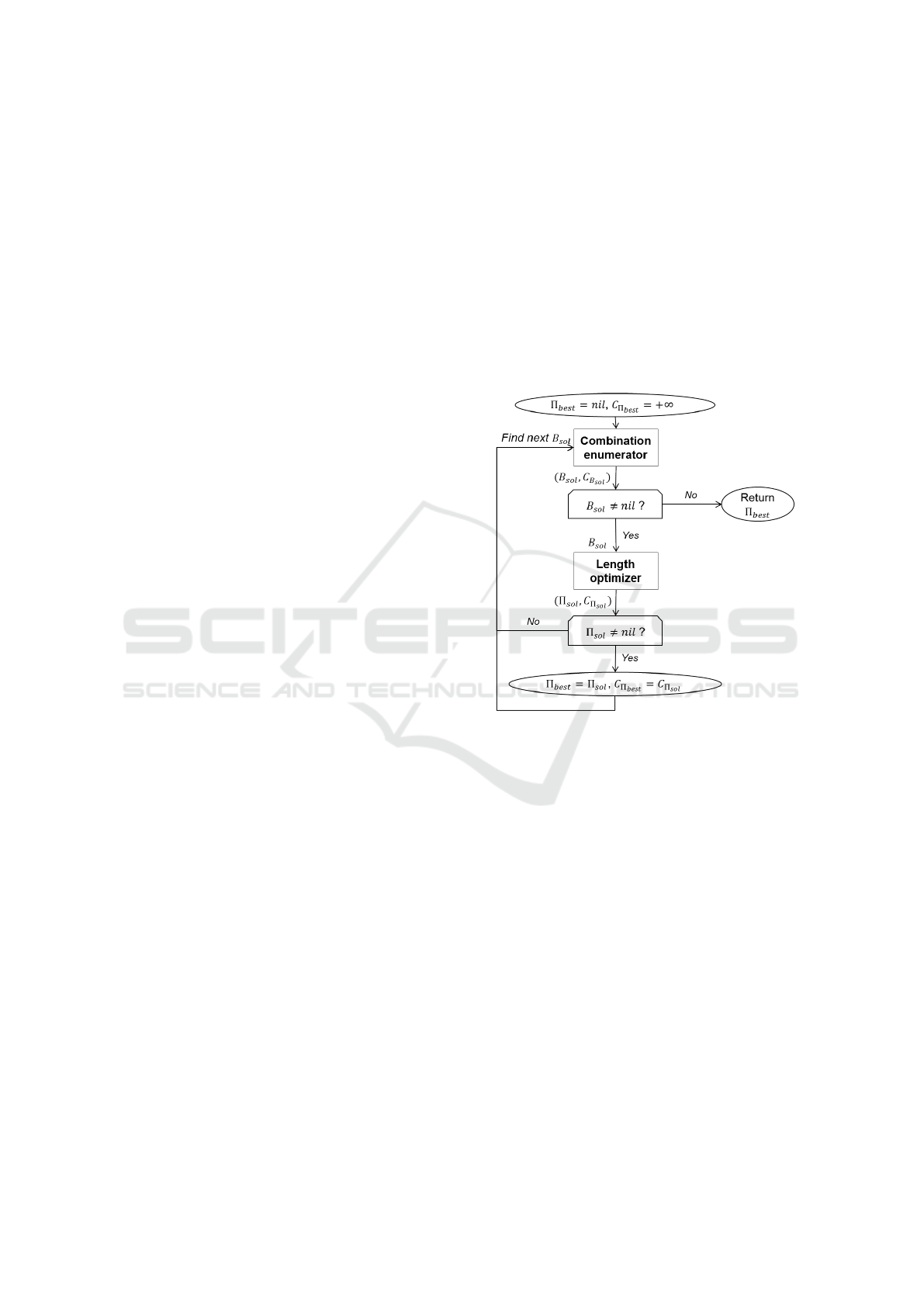
3.2 Problem Decomposition
To solve the 3D-OFPRP, we use a decomposition ap-
proach that exploits two solvers, as shown in Fig-
ure 5. The first solver, called combination enumer-
ator, enumerates the possible bend combinations B
sol
containing N
B
sol
∈
{
0,..., N
max
}
bends of catalog B
cat
and ensuring that the destination configuration can be
reached from the source configuration. Combination
B
sol
can also be the empty combination here (case
N
B
sol
= 0). The second solver, called length optimizer,
takes as an input a bend combination B
sol
produced
by the combination enumerator and computes the op-
timal route Π
sol
for B
sol
. This optimal route is com-
puted through a linear program that finds the optimal
length of straight sections between each pair of bends.
This way, by iterating between the two solvers, it is
possible to compute the optimal pipe route.
As soon as the combination enumerator does not
have any more solution (see the branching on condi-
tion B
sol
6= nil in Figure 5) the current best solution
pipe Π
best
is returned. Otherwise, the length opti-
mizer is called to find a solution which is better than
Π
best
. When the length optimizer finds such a solution
Π
sol
, Π
best
is updated. The combination enumerator
is then requested for the next possible bend combina-
tion.
Figure 5: Architecture of the solver.
The time complexity of this 2-step pipe routing
algorithm corresponds to the time complexity of the
combination enumerator multiplied by the time com-
plexity of the length optimizer which, as shown in
Section 3.4, is based on a linear program solvable in
polynomial time.
3.3 Combination Enumerator
The combination enumerator enumerates the bend
combinations B
sol
that allow to reach the destination
orientation from the source orientation using at most
N
max
bends of catalog B
cat
. It is an enumeration
solver: for an instance of a bend combination prob-
lem between o
s
(corresponding to orientation R
s
) and
o
d
(corresponding to orientation R
d
), at each request,
the solver returns a possible bend combination which
has not been previously returned, if such a combina-
tion exists.
To do so, the bend combination problem is formu-
lated as a reachability problem in the reachable orien-
Optimal Pipe Routing Techniques in an Obstacle-Free 3D Space
73
tation graph G(O, E). For this reachability problem,
the revisit of a node is allowed in order to have a com-
plete enumeration of the possible bend combinations.
A bend combination can indeed contain several times
the same orientation o ∈ O as a transition orientation.
The enumeration algorithm is an A* search algorithm
based on successive calls to the following procedure,
starting with the list OpenList of combinations to ex-
plore, initialized with the empty combination. This
procedure is presented in Algorithm Find next B
sol
.
To avoid the exploration of the uninteresting bend
combinations, a lower bound C
LB
(B) of the best pipe
route which can be obtained with bend combination
B is used. This way, the bend combinations B such
that C
LB
(B) is greater than or equal to the current best
pipe cost C
Π
best
are not explored. A valid lower bound
takes into account the cost of the bend combination
and the minimal cost of the straight sections:
C
LB
(B) = max
C
B
+ (N
B
+ 1)αL
min
, αk
−−→
P
s
P
d
k
In the previous expression, we implicitly assume that
using a unique straight section cannot be more costly
than using bends. The bound proposed could be made
tighter by considering the minimum cost of the bends
required to reach the goal orientation in the reachable
orientation graph.
Furthermore, the list OpenList of bend combina-
tions to explore is sorted by increasing order of lower
bounds C
LB
(·). To do this, each time a new bend
combination B must be added to OpenList, its corre-
sponding bound C
LB
(B) is computed so that it can be
inserted at the right position in the list. Then, function
PopFirstElement used in Algorithm 1 removes and re-
turns a bend combination B whose C
LB
(·) value is the
lowest, which allows to explore the more promising
bend combinations first.
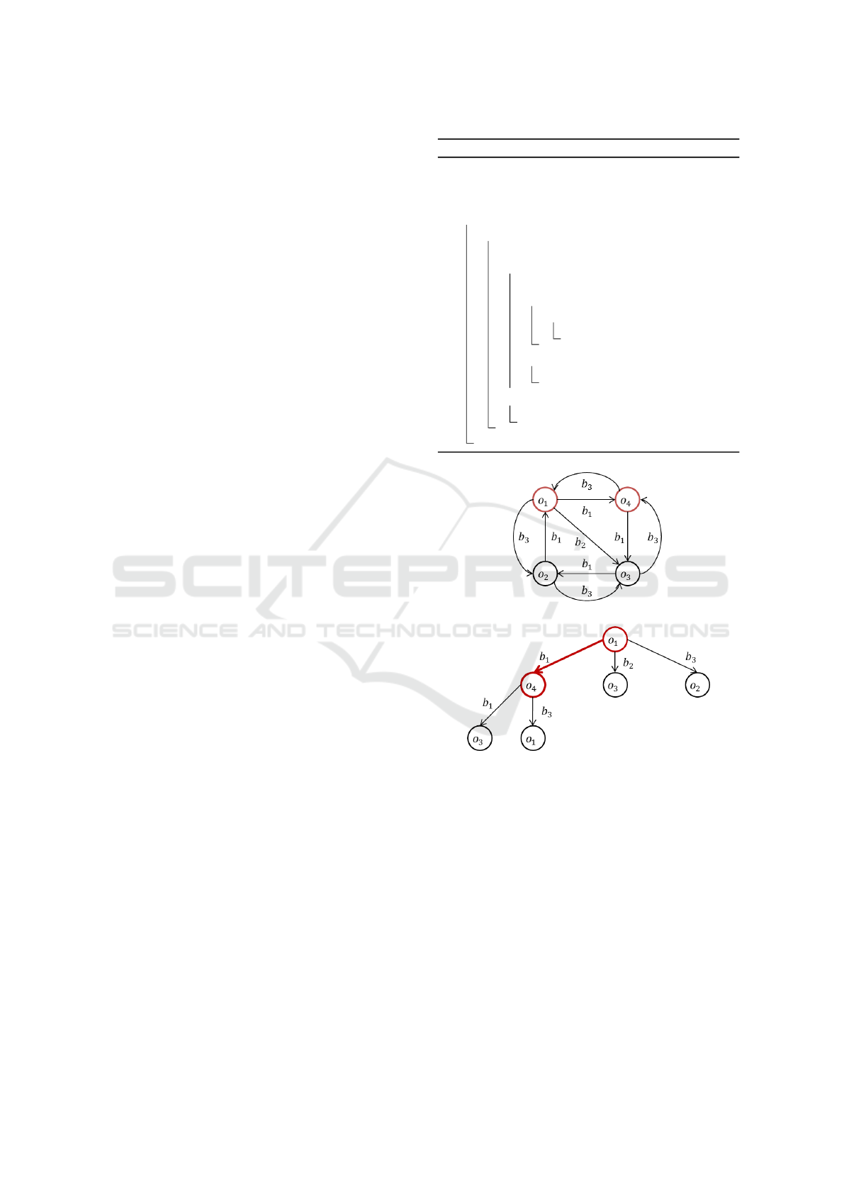
Figure 6 shows the evolution of the search tree for
a simple reachable orientation graph containing 4 ori-
entations and 3 bends such that C
b
1
< C
b
2
< C
b
3
<
2C
b
1
, with orientation o
1
as source orientation and
orientation o
4
as destination orientation. In this case,
for N
max
= 2, the procedure returns bend combina-
tion B
1
= [b
1
] on the first call and bend combination
B
2
= [b
2
,b
3
] on the second one. For N
max
= 4, a
bend combination such as [b
1
,b
1
,b
3
] traversing ori-
entations [o
1
,o
4
,o
3
,o
4
] could also be returned.
It can be noted that at this step, both the bend cata-
log constraints (Section 2.2.2) and the pipe attachabil-
ity constraints (Section 2.2.3) are taken into account.
3.4 Length Optimizer
The length optimizer defines the 3D-route of the pipe
for a given bend combination B
sol
= [b
1
,..., b
n
] by
Algorithm 1: Find next B
sol
.
Data: G (O,E), OpenList, o
s
, o
d
, C
Π
best
,
N
Max
≥ 0
Result: B
sol
begin
while OpenList 6=
/
0 do
B ← PopFirstElement (OpenList)
if C
LB
(B) < C
Π
best
then
o
B
← B (o
s
)
if N
B
< N
Max
then
for (o
B
,b, o) ∈ E do
Add B ∪ [b] to OpenList
if o
B
= o
d
then
return B
else
return nil
return nil
(a) Reachable orientation graph G(O, E).
(b) First solution.
Figure 6: Example of bend combination enumeration.
computing the length of the straight sections. As the
bend combination is known, the orientations O
i
= R
T
i
of each transition configurations can be calculated.
Then, the 3D-OFPRP with a given bend combi-
nation B
sol
can be formulated as an LP problem that
contains two types of variables:
• the length variables `
i
such that, for i ∈
{
0,..., n
}
,
real variable `
i
is the length of the i
th
straight sec-
tion (see Figure 7);
• the transition point variables
−→
p
i
= (p
x
i
, p
y
i
, p
z
i
)
such that, for i ∈
{
0,..., n + 1
}
, real variable p
x
i
(respectively p
y
i
and p
z
i
) is the coordinate of tran-
sition point p
T
i
(see Figure 7) on the X-axis (re-
ICORES 2020 - 9th International Conference on Operations Research and Enterprise Systems
74

spectively on the Y -axis and on the Z-axis).
Figure 7: Indices of the transition points, lengths and bends
for a 2-bend pipe.
The linear problem to solve is then:
minimize
n
∑
i=0
α`
i
(8)
subject to:
−→
p
0
=
−→
p
s
(9)
−−→
p
n+1
=
−→
p
d
(10)
∀i ∈
{
0,..., n + 1
}
, ∀ j ∈
{
1,..., k
A
}
,
A
j
p
x
i
+ B
j
p
y
i
+C
j
p
z
i
+ D
j
≤ 0 (11)
∀i ∈
{
0,..., n
}
, `
i
≥ L
min
(12)
∀i ∈
{
1,..., n + 1
}
,
−→
p
i
=
−−→
p
i−1
+
`
i−1
+ L
b
i−1
+ L
b
i
−−→
z
O
i−1
(13)
C
B
sol
+
n
∑
i=0
α`
i
≤ C
Π
best
− 1 (14)
∀i ∈
{
0,..., n
}
, `
i
∈ R
+
(15)
∀i ∈
{
0,..., n + 1
}
,
−→
p
i
∈ R
3
(16)
Constraints 9 and 10 are the origin and destination
constraints. Constraints 11 are the routing space con-
straints. Constraints 12 model the minimal straight
section length constraints. Last, Constraints 13 are
the position succession constraints. In this equa-
tion, terms L
b
i−1
and L
b
i
represent respectively the
cost contribution of the half lengths of the previous
and next bends to the length of the segment between
transition points i − 1 and i, and with the convention
L
b
0
= 0 and L
b
n+1
= 0. Last, Constraint 14 forces to
find a solution that is strictly better than the best solu-
tion known (Π
best
).
Contrarily to most of the existing algorithms, such
an LP formulation allows to route in a continuous 3D
space. In particular, it does not restrain the pipe route
to candidate paths using nodes in a discretized 3D rep-
resentation.
This part of the combined solver takes into ac-
count the spatial constraints, including the routing
space constraints and the design constraints about
straight sections. It is also responsible for optimizing
the straight section part of the criterion.
4 MILP MODEL
The second method proposed in this paper is based on
a MILP formulation of the 3D-OFPRP(n) problem,
which also uses the transition points and the graph of
reachable orientations G (O,E). More precisely, the
problem contains four types of variables :
• the bend variables x
i,b
such that, for i ∈
{
1,..., n
}
,
integer variable x
i,b
equals 1 if the i
th
bend of the
pipe (see Figure 7) is bend b ∈ B
cat
, 0 otherwise;
• the length variables `
i
such that, for i ∈
{
0,..., n
}
,
real variable `
i
is the length of the i
th
straight sec-
tion;
• the transition orientation variables y
i,o
such that,
for i ∈
{
0,..., n
}
, integer variable y
i,o
equals 1 if
the orientation of transition configuration T
i
is ori-
entation o ∈ O, 0 otherwise;
1
• the transition point variables
−→
p
i
= (p
x
i
, p
y
i
, p
z
i
)
such that, for i ∈
{
0,..., n + 1
}
, real variable p
x
i
(respectively p
y
i
and p
z
i
) is the coordinate of tran-
sition point p
T
i
on the X-axis (respectively on the
Y -axis and on the Z-axis).
This way, the 3D-OFPRP(n) can be formulated as
the following Mixed Integer Linear Program:
minimize
n
∑
i=1
∑
b∈B
cat
x
i,b
C
b
+
n
∑
i=0
α`
i
(17)
subject to:
∀i ∈
{
1,..., n
}
,
∑
b∈B
cat
x
i,b
= 1 (18)
∀i ∈
{
0,..., n
}
,
∑
o∈O
y
i,o
= 1 (19)
y
0,o
s
= 1 (20)
y
n,o
d
= 1 (21)
−→
p
0
=
−→
p
s
(22)
−−→
p
n+1
=
−→
p
d
(23)
∀i ∈
{
0,..., n + 1
}
, ∀ j ∈
{
1,..., k
A
}
,
A
j
p
x
i
+ B
j
p
y
i
+C
j
p
z
i
+ D
j
≤ 0 (24)
∀i ∈
{
0,..., n
}
, `
i
≥ L
min
(25)
∀i ∈
{
1,..., n + 1
}
, ∀o ∈ O,
−→
p
i
≤
−−→
p
i−1
+ (`
i−1
+ L (i))
−→
z
o
+
−→
M (1 − y
i−1,o
) (26)
1
The use of such variables reduces the number of vari-
ables compared to a formulation that would use variables
x
i,o,b
∈ {0,1} taking value 1 if and only if the i
th
bend of
the pipe is bend b and the orientation of i
th
transition point
is orientation o.
Optimal Pipe Routing Techniques in an Obstacle-Free 3D Space
75

∀i ∈
{
1,..., n + 1
}
, ∀o ∈ O,
−→
p
i
≥
−−→
p
i−1
+ (`
i−1
+ L (i))
−→
z
o
−
−→
M (1 − y
i−1,o
) (27)
∀i ∈
{
1,..., n
}
, ∀o ∈ O,
∀b ∈ B
cat
| 6 ∃o
0
∈ O
o,b, o
0
∈ E,
y
i−1,o
+ x
i,b
≤ 1 (28)
∀i ∈
{
1,..., n
}
, ∀o
0
∈ O,
∀b ∈ B
cat
| 6 ∃o ∈ O
o,b, o
0
∈ E,
x
i,b
+ y
i,o
0
≤ 1 (29)
∀i ∈
{
1,..., n
}
, ∀o ∈ O,
∀o
0
∈ O | 6 ∃b ∈ B
cat
o,b, o
0
∈ E,
y
i−1,o
+ y
i,o
0
≤ 1 (30)
∀i ∈
{
1,..., n
}
, ∀
o,b, o
0
∈ E,
x
i,b
+ y
i−1,o
≤ 1 + y
i,o
0
(31)
y
i,o
0
+ x
i,b
≤ 1 + y
i−1,o
(32)
y
i−1,o
+ y
i,o
0
≤ 1 + x
i,b
(33)
∀i ∈
{
1,..., n
}
, ∀b ∈ B
cat
x
i,b
∈
{
0,1
}
(34)
∀i ∈
{
0,..., n
}
, `
i
∈ R
+
(35)
∀i ∈
{
0,..., n
}
, ∀o ∈ O y
i,o
∈
{
0,1
}
(36)
∀i ∈
{
0,..., n + 1
}
,
−→
p
i
∈ R
3
(37)
Constraints 18 and 19 ensure respectively the bend
and the transition orientation unicity. Constraints 20
and 21 are the origin and destination constraints for
the orientation. Constraints 22-25 are the same as in
the LP formulation. Constraints 26-27 are the posi-
tion succession constraints. The successive transition
points are defined using a big-M formulation that en-
sures that transition point
−→
p
i
corresponds to the previ-
ous transition point
−−→
p
i−1
translated along the previous
transition orientation
−−→
z
o
i−1
. The translation distance
takes into account the previous straight section length
`
i−1
and the half lengths of the previous bend i − 1
and of bend i, if they exist. Term
−→
M ∈ (R
+
)
3
is an
arbitrary value that should be greater than the bigger
dimension of the routing space in order not to reduce
the possible positions for each transition point. More-
over, to simplify Constraints 26-27, term L (i) is de-
fined by:
L (i) = L
−
(i) + L
+
(i)
where:
L
−
(i) =
∑
b∈B
cat
x
i−1,b
L
b
if i > 1
0 otherwise
L
+
(i) =
∑
b∈B
cat
x
i,b
L
b
if i < n + 1
0 otherwise
Constraints 28-30 avoid the use of bend-orientation
triplets (o,b, o
0
) ∈ O × B
cat
×O which do not match a
possible arc in the reachable orientation graph. This
formulation of the constraints with three parts gener-
ates less constraints than a formulation with only one
constraint y
i−1,o
+ y
i,o
0
+ x
i,b
≤ 2. Last, Constraints
31-33 are the orientation succession constraints. This
formulation ensures that if at least two elements of
bend-orientation triple (o,b, o
0
) ∈ E are chosen for the
i
th
segment of the pipe, then the last one is also cho-
sen. This supposes that there exists at most one bend b
such that (o,b, o
0
) ∈ E, which is true if all the bends of
B
cat
have different rotation matrices. If this hypothe-
sis is not verified, Constraints 31-33 can be removed.
5 RESULTS
The MILP approach and the Combined Graph-LP ap-
proach have been compared on four realistic test cases
requiring different numbers of bends to be solved.
5.1 Test Cases
The test cases are as follows:
• Case 1 contains source and destination in the
same plane with the same orientation and has a
2-bend optimal solution (see Figure 8a).
• Case 2 contains source and destination in differ-
ent planes with a rotated orientation along the Z-
axis and has a 3-bend optimal solution (see Figure
8b).
• Case 3 contains source and destination in differ-
ent planes with the same orientation and has a 4-
bend optimal solution (see Figure 8c).
• Case 4 contains source and destination in differ-
ent planes with a rotated orientation along the Z-
axis and destination at the back of the source. This
case has a 5-bend optimal solution (see Figure
8d).
The minimal length of the straight sections used is
L
min
= 2. The routing space is a cube of width 10000
centered in (0, 0,0). The linear cost of straight sec-
tions is α = 1.
The four test cases have been solved with three
different bend catalogs containing bends around the
X-axis and Y -axis (no twisted section around the Z-
axis in the catalogs). The first catalog B
cat.1
contains
four orthogonal bends (N
B
cat.1
= 4). The second one
B
cat.2
contains the four orthogonal bends and four 45
◦
ICORES 2020 - 9th International Conference on Operations Research and Enterprise Systems
76
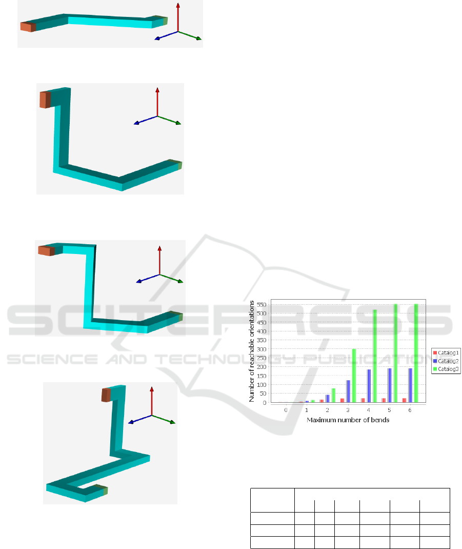
(a) Case 1 (source:(0, 0,0), destination: (3000,−2000, 0),
same orientation for the source and the destination).
(b) Case 2 (source:(0,0, 0), destination:
(3000,−2000, 2000), rotated orientation along the
Z-axis for the source and the destination).
(c) Case 3 (source:(0,0, 0), destination:
(3000,−2000, 2000), same orientation for the source
and the destination).
(d) Case 4 (source:(0,0, 0), destination:
(−3000,−2000, 2000), rotated orientation along the
Z-axis for the source and the destination, and destination
at the back of the source).
Figure 8: Test cases with catalog B
cat.3
, with for each test
case the (x,y,z) coordinates of the source and the destina-
tion.
bends (N
B
cat.1
= 8). The last one B
cat.3
contains the
four orthogonal bends, four 30
◦
bends and four 60
◦
bends (N
B
cat.3
= 12).
In order to minimize the number of bends first
and then the total length, all the bends have a cost of
20000 which is high compared to the euclidean dis-
tance between the source and the destination.
5.2 Generation of the Reachable
Orientations
The graph of reachable orientations has been gener-
ated for each catalog. Figure 9 shows, for each bend
catalog, the evolution of the number of reachable ori-
entations with the maximum number of bends N
max
allowed in a pipe.
It should be noted that the number of reachable
orientations has an asymptotic trend when the number
of bends grows. This is explained because first the
attachability constraint is taken into account during
the enumeration, and second there is a finite number
of possible orientations in a given plane due to the
bend catalog. In the end, the number of reachable
orientations is quite small and the enumeration is easy
and fast, as shown in Table 1 which presents average
times obtained on 10 generations of graph G (O, E)
for each catalog.
Figure 9: Evolution of the number of reachable orientations
with the number of bends for each catalog.
Table 1: Average time required to generate the reachable
orientation graph (in milliseconds).
Catalog
Maximum number of bends
1 2 3 4 5 6
B
cat.1
2. 1. 2. 2. 2. 1.
B
cat.2
0. 1. 6. 18. 27. 32.
B
cat.3
0. 1. 24. 185. 310. 303.
5.3 Comparison of Both Approaches
The MILP model has been implemented using the
OPL language and the instances have been solved us-
ing CPLEX 12.9 with an Intel Xeon 1.90 GHz pro-
cessor and 64 GB RAM. The Combined Graph-LP
solver has been implemented in Java and uses the LP
Optimal Pipe Routing Techniques in an Obstacle-Free 3D Space
77
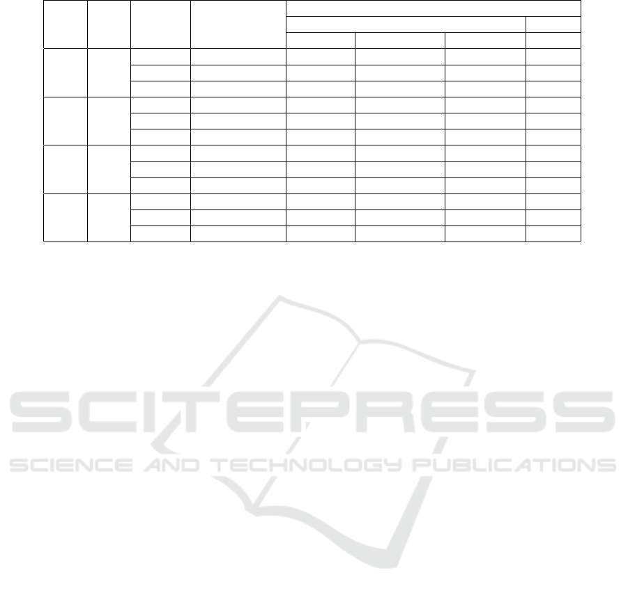
Table 2: Results of the Combined Graph-LP and MILP approaches.
Case N
max
Catalog Optimal value
Average time to optimum (in s)
Combined Graph-LP MILP
Total Comb.Enum. Len.Optim. Total
1 2
B
cat.1
43400 0.118 0.025 0.093 0.304
B
cat.2
43165.69 0.028 0.017 0.011 2.571
B
cat.3
43230.94 0.024 0.011 0.013 1.265
2 3
B
cat.1
64600 0.013 0.006 0.007 0.324
B
cat.2
64600 0.053 0.047 0.006 0.681
B
cat.3
64600 0.162 0.153 0.009 2.321
3 4
B
cat.1
83800 0.058 0.013 0.045 10.435
B
cat.2
83565.69 1.000 0.939 0.061 12.606
B
cat.3
83630.94 13.413 13.303 0.110 9.693
4 5
B
cat.1
105400 0.207 0.126 0.081 29.873
B
cat.2
105400 45.747 45.574 0.173 27.369
B
cat.3
105400 2573.032 2572.765 0.267 28.385
solver of the Apache Commons Math 3.6.1 library
with an Intel 2.70GHZ precessor and 16 GB RAM.
As the complexity of this approach comes from the
enumeration of bend combinations, the use of the LP
solver of Apache Commons Math 3.6.1 rather than
CPLEX 12.9 has no significant impact on computa-
tion times. Both solvers have been run on the four test
cases with the different catalogs. The results of the
Combined Graph-LP solver and of the MILP model
are shown in Table 2 which presents the average com-
putation times obtained on 5 executions for each cat-
alog.
Both approaches find the optimal solutions and
prove the optimality on each test case. Although the
MILP model is slower than the Combined Graph-LP
solver with a small number of bends N
max
or small
catalog size N
B
cat
, the MILP approach is more ro-
bust when N
max
and N
B
cat
increase. Actually, for
small problem instances, the resolution is immedi-
ate for both methods, but the initialization time of the
MILP model (time before the search actually starts) is
greater than the initialization time of the Linear Pro-
gram with fixed bends. Then, it can be noticed that
when the bends added to the catalog allow to improve
the optimal solution, the resolution of the MILP is
faster even if the problem instance contains more vari-
ables. This is due to better cuts in the MILP resolution
which avoid to unnecessarily consider branches of the
search space. There is no equivalent mechanism in the
Combined Graph-LP solver. Furthermore, the num-
ber of bend combinations to explore in the Combined
Graph-LP solver is in O
(N
B
cat
)
N
max
and increases
exponentially with N
max
as shows the time spent in
Combination Enumerator in Table 2.
5.4 Discussion
Both approaches are based on the enumeration of
reachable orientations. This enumeration can be time-
consuming with large bend catalogs and without pipe
orientation constraints to limit the admissible orien-
tations. In this case, if several pipes must be routed
based on the same catalog, the enumeration can be
done only once by considering relative routing prob-
lems that express the destination, the routing space
and the reachable orientations relatively to the origin
pipe configuration which is assimilated to the refer-
ence of the 3D coordinates system.
Furthermore, with test cases 1 and 3, it can be no-
ticed that the introduction of non orthogonal bends
in the catalog, such as 30
◦
, 45
◦
or 60
◦
bends, reduces
the cost of the optimal solution by saving length. This
shows that extending existing pipe routing approaches
by using non orthogonal bends is relevant. Other cat-
alogs using only non orthogonal bends (e.g. a catalog
containing only the 30
◦
, 45
◦
, and 60
◦
bends) could
also be tested. Also, approaches using bend catalogs
can easily be extended to the use of more complex
patterns with several transition configurations, which
is profitable for the reuse of existing patterns in the
providers’ catalog.
6 CONCLUSIONS AND
PERSPECTIVES
This paper introduced two approaches to route a pipe
in a 3D continuous space using bends from a catalog.
Bends can be described by a rotation matrix and can
be non orthogonal. Both approaches are based on the
enumeration of reachable orientations at a preprocess-
ICORES 2020 - 9th International Conference on Operations Research and Enterprise Systems
78

ing step, which takes into account the orientation of
the source and destination sections of the pipe. Also,
the techniques proposed make pipe routing possible
for pipes that have a non symmetrical section such as
a rectangular one.
Both presented approaches are sensitive to the in-
crease in the number of bends, even if the MILP ap-
proach seems more robust for delivering an optimal
solution. The MILP resolution might also be boosted
by using column generation techniques with a master
problem considering bend variables. The Combined
Graph-LP solver could also be accelerated by im-
proving the combination enumeration procedure with,
for example, a bidirectional A* enumeration starting
from the source and destination orientations.
As a result, the new methods introduced in this
paper can be efficiently used as a first routing algo-
rithm. If the optimal pipe route obtained by solving
the 3D-OFPRP problem collides with obstacles of the
3D-PRP problem, Branch-and-Cut techniques can be
integrated to the MILP approach by (a) analyzing the
solution generated, (b) adding new integer variables
and new linear constraints to enforce that pipe sec-
tions must not traverse the obstacle sides for which
collisions are detected, (c) solving the problem again,
and so on until a valid pipe routing is found. One dif-
ficulty though will concern the management of colli-
sions with the pipe itself, since the pipe sections can-
not be considered as fixed obstacles from one resolu-
tion to the next.
REFERENCES
Ando, Y. and Kimura, H. (2012). An automatic piping al-
gorithm including elbows and bends. Journal of the
Japan Society of Naval Architects and Ocean Engi-
neers, 15:219–226.
Asmara, A. and Nienhuis, U. (2006). Automatic piping sys-
tem in ship. In International Conference on Computer
and IT Application (COMPIT).
Belov, G., Czauderna, T., Dzaferovic, A., de la Banda,
M. G., Wybrow, M., and Wallace, M. (2017). An op-
timization model for 3d pipe routing with flexibility
constraints. In International Conference on Princi-
ples and Practice of Constraint Programming, pages
321–337. Springer.
Fan, X., Lin, Y., and Ji, Z. (2006). The ant colony opti-
mization for ship pipe route design in 3d space. In
2006 6th World Congress on Intelligent Control and
Automation, pages 3103–3108. IEEE.
Furuholmen, M., Glette, K., Hovin, M., and Torresen,
J. (2010). Evolutionary approaches to the three-
dimensional multi-pipe routing problem: a compar-
ative study using direct encodings. In European Con-
ference on Evolutionary Computation in Combinato-
rial Optimization, pages 71–82. Springer.
Guirardello, R. and Swaney, R. E. (2005). Optimization of
process plant layout with pipe routing. Computers &
chemical engineering, 30(1):99–114.
Hightower, D. W. (1969). A solution to line-routing prob-
lems on the continuous plane. In Proceedings of the
6th annual Design Automation Conference, pages 1–
24. ACM.
Ikehira, S., Kimura, H., Ikezaki, E., and Kajiwara, H.
(2005). Automatic design for pipe arrangement us-
ing multi-objective genetic algorithms. Journal of the
Japan Society of Naval Architects and Ocean Engi-
neers, 2:155–160.
Ito, T. (1999). A genetic algorithm approach to piping route
path planning. Journal of Intelligent Manufacturing,
10(1):103–114.
Jiang, W.-Y., Lin, Y., Chen, M., and Yu, Y.-Y. (2015). A co-
evolutionary improved multi-ant colony optimization
for ship multiple and branch pipe route design. Ocean
Engineering, 102:63–70.
Kimura, H. (2011). Automatic designing system for pip-
ing and instruments arrangement including branches
of pipes. In International Conference on Computer
Applications in Shipbuilding (ICCAS), pages 93–99.
IEEE.
Lee, C. Y. (1961). An algorithm for path connections and its
applications. In IRE transactions on electronic com-
puters, number 3, pages 346–365. IEEE.
Liu, L. and Liu, Q. (2018). Multi-objective routing of multi-
terminal rectilinear pipe in 3d space by moea/d and
rsmt. In 3rd International Conference on Advanced
Robotics and Mechatronics (ICARM), pages 462–467.
IEEE.
Medjdoub, B. and Bi, G. (2018). Parametric-based dis-
tribution duct routing generation using constraint-
based design approach. Automation in Construction,
90:104–116.
Park, J.-H. and Storch, R. L. (2002). Pipe-routing algorithm
development: case study of a ship engine room design.
Expert Systems with Applications, 23(3):299–309.
S.-H., K., W.-S., R., and S., J. B. (2013). The develop-
ment of a practical pipe auto-routing system in a ship-
building cad environment using network optimization.
International journal of naval architecture and ocean
engineering, 5(3):468–477.
Sakti, A., Zeidner, L., Hadzic, T., Rock, B. S., and Quar-
tarone, G. (2016). Constraint programming approach
for spatial packaging problem. In International Con-
ference on AI and OR Techniques in Constraint Pro-
gramming for Combinatorial Optimization Problems,
pages 319–328. Springer.
Zhu, D. and Latombe, J.-C. (1991). Pipe routing-path plan-
ning (with many constraints). In Proceedings. 1991
IEEE International Conference on Robotics and Au-
tomation, pages 1940–1947. IEEE.
Optimal Pipe Routing Techniques in an Obstacle-Free 3D Space
79
