Simultaneous Visual Context-aware Path Prediction
Haruka Iesaki
1
, Tsubasa Hirakawa
1
, Takayoshi Yamashita
1
, Hironobu Fujiyoshi
1
,
Yasunori Ishii
2
, Kazuki Kozuka
2
and Ryota Fujimura
2
1
Computer Science, Chubu University, 1200 Matsumoto-cho, Kasugai, Aichi, Japan
2
Panasonic Corporation, Japan
Keywords:
Path Prediction, Visual Forecasting, Predictions by Dashcams, Convolutional LSTM.
Abstract:
Autonomous cars need to understand the environment around it to avoid accidents. Moving objects like
pedestrians and cyclists affect to the decisions of driving direction and behavior. And pedestrian is not always
one-person. Therefore, we must know simultaneously how many people is in around environment. Thus, path
prediction should be understanding the current state. For solving this problem, we propose path prediction
method consider the moving context obtained by dashcams. Conventional methods receive the surrounding
environment and positions, and output probability values. On the other hand, our approach predicts proba-
bilistic paths by using visual information. Our method is an encoder-predictor model based on convolutional
long short-term memory (ConvLSTM). ConvLSTM extracts visual information from object coordinates and
images. We examine two types of images as input and two types of model. These images are related to people
context, which is made from trimmed people’s positions and uncaptured background. Two types of model are
recursively or not recursively decoder inputs. These models differ in decoder inputs because future images
cannot obtain. Our results show visual context includes useful information and provides better prediction re-
sults than using only coordinates. Moreover, we show our method can easily extend to predict multi-person
simultaneously.
1 INTRODUCTION
Paths prediction is strongly required by many applica-
tions (e.g., autonomous driving, robot navigation, and
congestion forecasts). In particular, there have been
many studies on autonomous driving. Autonomous
driving needs high precision performance in complex
environments. Thus, scene understanding is needed
to perceive the environment around the car. Scene un-
derstanding has rapidly progressed over the last few
years. It has been used to interpret risky regions
(Kozuka and Niebles, 2017), (Zeng et al., 2017a) and
visual explanations (Fukui et al., 2019), (Xu et al.,
2015). Scene understanding is needed for long-time
prediction because vehicles move at high speed. But
people are affected by many factors such as the scene
environment, road signs, human-human interactions,
and people’s beliefs. Therefore, predicting the hidden
states of people is necessary to predict people’s paths.
We represent the hidden state as the probability dis-
tributions from the driver’s viewpoint for the future.
Probability is the key to prevent collisions by predict-
ing future action to ensure safe driving on the road
because probability values can show how the risk in
the prediction areas.
Inspired by representation-based scene under-
standing methods, we propose an approach to pre-
dict the paths of people (including pedestrians and cy-
clists) by using dashcams in long-time horizons with
uncertainty estimates.
Our contributions are as follows:
• For scene understanding, previous methods are
image generation, risky region interpretation, and
visual explanation. We apply these methods to
path prediction by using dashcams.
• The surrounding environment can represent vari-
ous data types like bounding box, segmentation,
and optical flow. We compare how using visual
context images can improve prediction. We com-
pare using visual context images with two types
of image: RGB and optical flow.
• In the future prediction, we do not know how vi-
sual context images can obtain. We compare two
types of model, which differ what context images
input to the predictor.

2 RELATED WORK
2.1 Vector-based Predictions
Path prediction methods by using vectors have been
proposed (Bhattacharyya et al., 2017), (Zhang et al.,
2019), (Du et al., 2018), (Deo and Trivedi, 2018),
(Kooij et al., 2014). These approaches use coordi-
nates or velocities to indicate the movement of the
prediction target as input data and prediction results.
(Bhattacharyya et al., 2017) proposed an on-board
path prediction method. This method inputs bound-
ing box information into an encoder-decoder based
network, and the output bounding box indicates the
future target location in a set of image coordinates.
They introduce odometry information (i.e., speed and
angle) as additional inputs, which enables us to pre-
dict paths under a dynamic environment.
In contrast to the vector-based prediction methods,
our method inputs image data representing target lo-
cations and probabilistically predicts target locations
in each set of image coordinates. Our method can ex-
plain how visual contexts have effective information
and how this is easily extended to predictions of mul-
tiple targets.
2.2 Image-based Predictions
Prediction methods using image data have also been
proposed not only for path predicition problems (Re-
hder et al., 2017), (Makansi et al., 2019) but also an-
other prediction problems (Palazzi et al., 2017), (Shi
et al., 2015), (Bazzani et al., 2017). Image-based path
prediction methods use feature values extracted by us-
ing a convolutional neural network (CNN) and the
bounding boxes of the prediction targets as inputs.
Then, these data are input to a deep neural network
(DNN) (Hinton and Salakhutdinov, 2006), which pre-
dicts future target locations.
However, convoluted image data have many fea-
ture values. Thus, those feature values and bounding
boxes inputted to the DNN cause a problem because
the precious features of the bounding box disappear.
An effective obtainment from the image method
has been proposed by using a probabilistic attention
sight (Palazzi et al., 2017), (Bazzani et al., 2017),
forecasting segmentation by using segmentation im-
ages (Luc et al., 2018), and probability prediction
of mixture probability distribution with images made
from trimmed people’s positions (Makansi et al.,
2019).
Methods to extract features from images have
been proposed (Tran et al., 2015), (Shi et al., 2015),
(Zeng et al., 2017b), (Hsieh et al., 2018). (Shi
h
t-1
Convolutional 2D
x
t
Convolutional 2D
+
+ + + +
σ σ σtanh
g
t
c
t
i
t
f
t
C
t-1
C
t
h
t
×
×
tanh
+×
h
t
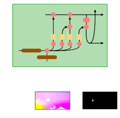
Figure 1: Convolutional Long Short-Term Memory (Con-
vLSTM).
Made Image
Input to Network
Optical Flow Image
+
=
Bounding Box
{(x
1
, y
1
), (x
2
, y
2
)}
Figure 2: Dataset sample image.
et al., 2015) proposed an encoder-predictor network
which is also called encoding-forecasting structure.
The encoder-predictor model consists of convolu-
tional long short-term memory (ConvLSTM). Con-
vLSTM is a recursive learning method with requiring
inputted image features. The ConvLSTM network we
used is shown in Figure 1. The ConvLSTM consists
of convolution layers and long term-short memory
(LSTM) (Hochreiter and Schmidhuber, 1997). Learn-
ing by LSTM usually needs inputted vectors such as
bounding box and odometry. On the other hand, Con-
vLSTM can use input images features. Input features
x
t
and previous hidden state’s features h
t−1
convo-
lute, and these features are separated into four LSTM
gates. ConvLSTM is able to extract image features
and learn recursively. This network can robustly pre-
dict paths for time sequence behavior.
3 PROPOSED METHOD
In this paper, we propose probabilistic paths predic-
tion by using captured dashcams images. We compare
two types of image and two types of model and, eval-
uate probability rates and the error which of truth and
prediction images. We explain the details of our pro-
posed method. Our approach also does not depends
on the number of people. Thus, we perform a one-
person prediction experiment and a multi-person pre-
diction experiment to verify this.
3.1 Context Images
The two types of image that are compared are RGB
and optical flow. RGB images are the ordinary im-

ages captured by dashcams. Optical flow images only
have information about movements surrounding ob-
jects. We use two types of image, which is made
from trimmed people’s positions, and the others back-
ground are uncaptured. They have only context about
people’s locations. A made image sample is shown in
Figure 2.
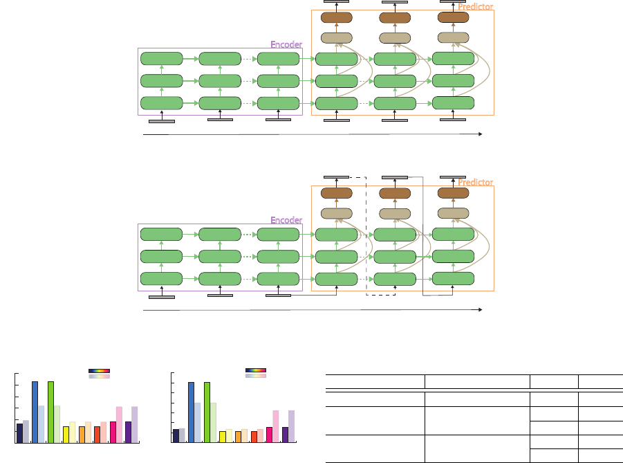
3.2 Network Architectures
The two types of models that are compared have dif-
ferent inputted decoder images. In this section, a non-
context image means black images.
Model 1
Model 1 is shown in Figure 3. A non-context im-
age is inputted to predictor each time. This model
only predict by using learned parameters in en-
coder. It means that how this model can predict
from visual context in the past.
Model 2
model 2 is shown in Figure 4. This model is re-
cursively input to predictor each time. The first
prediction uses the last image of the encoder, and
the others prediction use predicted images of each
previous time. We verify how the input image
in predictor effect to predict between the model
1 and model 2.
3.3 Training Loss
The training loss in learning time is the mean absolute
error (MAE) between a truth image and a prediction
image, as shown in Eq. 1. The number of prediction
frames is F, the batch size is B, a truth image is y, and
a prediction image is ˆy.
MAE =
1
B
1
F
B
∑
b=0
F
∑
f =0
(y, ˆy)
f
(1)
4 EXPERIMENTS
First, we evaluate the one-person path prediction in
4.3. Second, we evaluate the multi-person path pre-
diction in 4.4.
4.1 Dataset
Both of the experiments use the Cityscapes Dataset
(Cordts et al., 2016). This dataset has first-person
view video whose sequence of length 1.8 second (30
frames) obtained by dashcams and bounding boxes.
The video resolution is 1024×2048 pixels. Bound-
ing boxes is automatically annotated using tracking
by detection method of (Tang et al., 2016). Anno-
tation were obtained using the Faster R-CNN based
method of (Zhang et al., 2017). The coordinates at
the top left (x
1
, y
1
) and the bottom right (x
2
, y
2
) are
shown for each person’s position.
We also use the Oxford Town Centre dataset
(Adam and Jules, 2019). We use only multi-person
prediction for evaluating because multi-person is
more complex problems. The dataset is a CCTV
video, obtained from a surveillance camera, includes
approximately 2,200 people.
We make context images by using images and
bounding boxes, as explained in 3.1. There are three
two of images: RGB and optical flow images con-
verted by FlowNet 2.0 (Ilg et al., 2017). We does not
use optical flow as vectors because we predict visual
representation paths. We use optical flow color im-
ages which is converted vector to color. Them, these
have 3 channels.
The optical flow rates are shown in Figure5a,
5b. This is only people’s location rates of cityscapes
dataset. This shows the target person’s movements
whose directions are represented by flow. We cal-
culate the rate of eight directions, which are go-
ing counter clockwise, east-northeast (ENE), north-
northeast (NNE), north-northwest (NNW), west-
northwest (WNW), west-southwest (WSW), south-
southwest (SSW), south-southeast (SSE), and east-
southeast (ESE). This analysis shows optical flow
rates does not differ on whether it is a one-person
dataset or a multi-person dataset in training and test-
ing.
4.2 Evaluation Metrics
In this paper, we evaluate the path prediction accuracy
by using two performance indicators. We use negative
log likelihood (NLL) (which indicates probability dis-
tribution error) and mean IoU (recall and precision).
The NLL evaluates the probabilistic differences
between a prediction and true probability distribution.
In our experiments, we normalize the output values to
keep the property of probability distribution by using
the maximum output values and evaluate one.
The mean IoU (mIoU) calculates the average rate
of prediction probability in a truth bounding box and
a prediction area. We evaluate it by using precision
and recall rate. The precision rate is the rate of truth
bounding box range to the predicted distribution. In
contrast, the recall rate is the rate of predicted distri-
bution to the truth bounding box range. High preci-
sion means predictive quality. And high recall means

t
t t
t
t
t
t
Figure 3: Model 1: Encoder is inputted context images. Predictor is inputted non-context images.
t
t
t
t
t
t
t
Figure 4: Model 2: Encoder is inputted context images. Predictor is inputted the last image of the encoder and predictions.
(a) One-person
(b) Multi-person
Figure 5: The distribution of optical flow in Cityscapes
dataset. Each graph shows distributions of (a) one-person
prediction and (b) multi-person prediction.
how well the prediction matches to the truth bound-
ing box range, namely completeness. Each rates is
calculated by using to the number of pixels over each
threshold in the bounding box. The threshold range is
from 0.0 to 1.0, which represents the probability.
4.3 One-person Prediction
First, we evaluate one-person prediction using the
Cityscapes Dataset. The number of training samples
is 6,792 videos, and the number of testing samples
is 3,523 videos. The learning time is 10 epochs, and
the mini-batch size is 2. We use the Adam optimizer,
of which the learning rate is 0.001. Both input im-
ages (observation) and prediction images (future) are
10 frames. The images size is 128×256 pixels. In this
experiment, we compare two types of model and two
types of image.
Table 1: NLL of predictive distribution.
Method Prediction frames Image NLL
LSTM-Bayesian 8 RGB 3.92
Our model 1 10
RGB 0.693
Flow 0.692
Our model 2 10
RGB 0.693
Flow 0.692
4.3.1 Probability Distribution Error
For evaluating the probability distribution error, we
use the model of (Bhattacharyya et al., 2017) as a
baseline model. The results are shown in Table 1.
All of the results are lower than the baseline model.
Among the images, using optical flow images lowered
the error. It show the optical flow has effective move-
ment context but the RGB images have noise context
for prediction. However, it is not big different no mat-
ter what model to predict between models.
4.3.2 mIoU
The mIoU is shown in Figure 6a, 6b; the horizontal
axis is the threshold range 0.0 to 1.0, and the vertical
axis is the precision or recall rate in each bounding
box average. The rate is calculated by the average
over every prediction frame and the number of test-
ing samples. From both results, the RGB images pre-
dict approximately the same lower probability in the
bounding boxe area. On the other hand, optical flow
images are able to predict higher probability in the

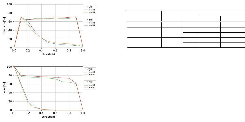
(a)
(b)
Figure 6: (a) Precision and (b) recall rates of one-person
prediction on Cityscapes dataset.
bounding box area. In the models using flow image,
recall is higher than precision when the threshold is
between 0.1 and 0.9. It show that these model predict
distribution close to truth bounding box area.
4.3.3 Visual Results for One-person
We show the only using optical flow images model in
Figure 7, 8, which is the highest accuracy in Figure
6b. Model 1 leads to a lower prediction than model
2 in the first time of prediction, show in Figure 7.
And Model 1 also predict distribution that is slightly
larger than the true value region. On the other hand,
Model 2 can predicts high probability distribution in
the truth bounding box area. In path prediction, model
1 is also the lower prediction, shown in Figure 8 but
both models predict approximately same paths. These
results show that the recursive input images of pre-
dictor (model 2) effects better to non-recursive model
(model 1) in the case of one-person prediction.
4.4 Multi-person Prediction
We also experiment on multi-person paths predic-
tion. It is a more complex problem than one-person
path prediction because people influence others ob-
jects. Therefor, we use the Cityscapes Dataset as we
did for the one-person prediction and Oxford Town
Centre Dataset. Cityscapes dataset’s training samples
are 1,978 videos, and the testing samples are 1,036
videos. The training conditions such as the learn-
ing time and the optimization are the same as those
of the one-person prediction. Town Centre dataset’s
Table 2: NLL of predictive distribution.
Method
Prediction
Image
NLL
frames Cityscapes Town centre
LSTM-Bayesian 8 rgb 3.92 -
Our model 1 10
rgb 0.692 0.670
flow 0.690 0.650
Our model 2 10
rgb 0.692 0.670
flow 0.690 0.650
training samples are 135 videos, and the testing sam-
ples are 57 videos. The condition is also same as ex-
periment using Cityscapes dataset, but image size is
135×240 pixels and the learning time is 200 epochs.
We also compare two models (non-recursive and re-
cursive predictor) and two types of image (RGB and
optical flow).
4.4.1 Probability Distribution Error
Models using optical flow image are the lower er-
ror than the baseline model, show in Table 2. This
does not show a big difference as to which model is
suitable for prediction. However, using Town Centre
dataset is lower than Cityscapes dataset. This is prob-
ably because Town Centre dataset is obtained by fixed
camera, so there are no rapidly movement samples.
4.4.2 mIoU
The mIoU is shown in Figure 9a, 9b, 10a, 10b. As
the results, RGB images predict almost the same low
probability in bounding box area, show in Figure 9a,
9b. On the other hand, models using optical flow im-
ages predict high probability in bounding box area.
In using optical flow models, the higher overlap rate
is in the order of model 2, 1. These results show us-
ing recursively context image have the better effect on
prediction than using non-context images. The mod-
els used Town Centre dataset is also almost same re-
sult, show in Figure 10a, 10b. However, predictions
with low threshold is high recall for both models and
images. This is thought to be because there is little
information on movement by flow obtained from the
bird’s-eye view.
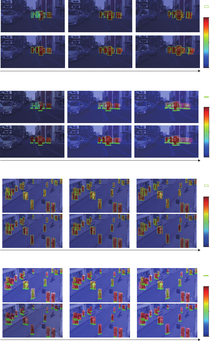
4.4.3 Visual Results for Multi-person Prediction
We show the only using optical flow images model
in Figure 11, 12, 13, 14, which is the highest ac-
curacy in Figure 9b, 10b. Figure 11, 12 are the re-
sults of Cityscapes dataset. Figure 13, 14 are the re-
sults of Town Centre dataset. Figure 11, 13 show the
probability prediction with truth bounding boxes for
each time. Figure 12, 14 show path predictions with
path defined the truth bottom bounding boxes as truth
paths. Both models gradually decrease the probability

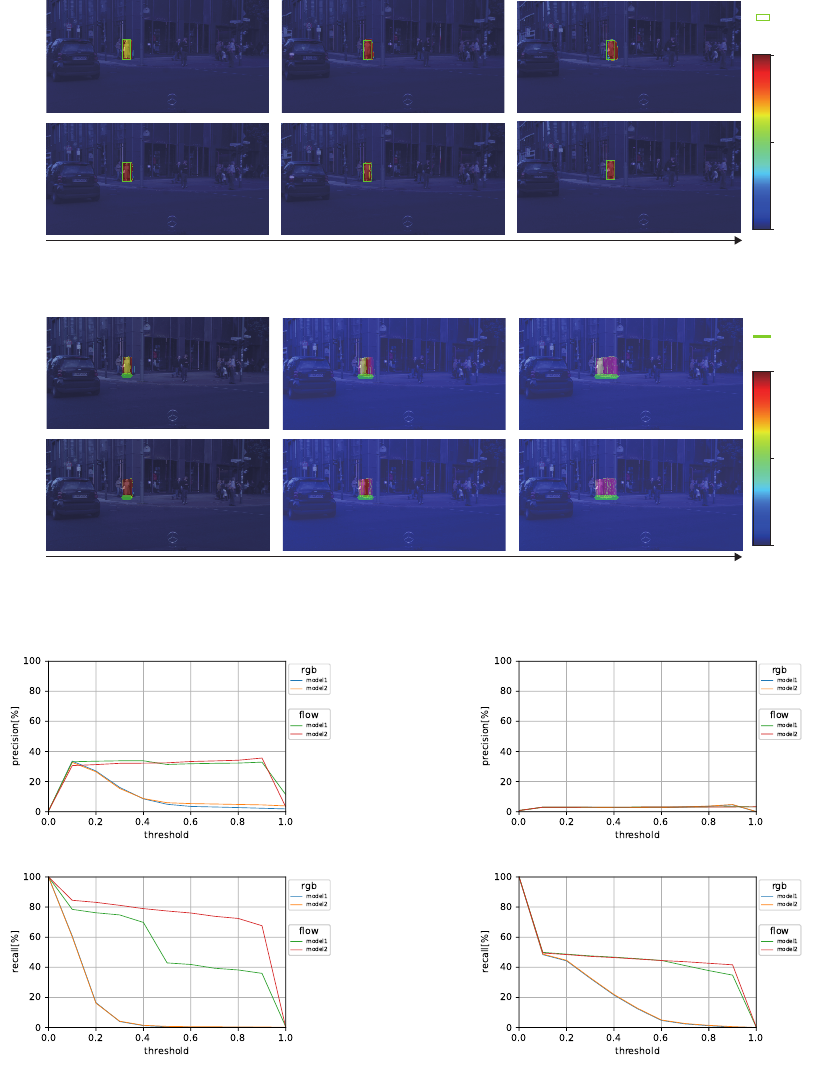
t
frames
t
t + 4 t + 9
Figure 7: Prediction results of one-person prediction on Cityscapes dataset.
t
frames
t t + 4 t + 9
Figure 8: Path prediction results of one-person prediction on Cityscapes dataset.
(a)
(b)
Figure 9: (a) Precision and (b) recall rates of multi-person
prediction on Cityscapes dataset.
in time sequence as shown in Figure11, 13. The rea-
son for the results seems to be that the learning fea-
tures in the encoder have disappeared in the predictor
as time has progressed. In using Cityscapes dataset,
(a)
(b)
Figure 10: (a) Precision and (b) recall rates of multi-person
prediction on Town Centre dataset.
model 2 predict high probability in the first predic-
tion compared to model 1. Predicted paths are over-
lap each other in progressing time, as show in Figure
12. However, paths are predicted low probability in

model 1. On the other hand, model 2 is able to predict
high probability until the last prediction time. The
model 2 using Town Centre dataset are also higher
prediction than model 1 in the first prediction time,
as shown Figure 13. Figure 14 shows all models are
predictable along each the truth path. From the above
results, recursive model (model2) can predict better
than non-recursive model (model 1).
5 CONCLUSIONS
We proposed a probabilistic paths prediction method
based on an encoder-predictor model. The proposed
method uses context images which visually represents
the state and movement of people’s positions. The
conventional encoder-predictor model applies to im-
ages generation. We applied it to paths prediction
with expressing probability distribution. We made
context images for getting effective information, and
evaluated two types of images and two models in one-
person and multi-person prediction. The experimen-
tal results show optical flow image can get better val-
ues than RGB images. And we also show that model
2, which input the last image of encoder and recur-
sively input images in predictor, is better than a non-
recursive model. Our future work includes planning
to predict individual paths in multi-person prediction.
REFERENCES
Adam, H. and Jules, L. (2019). Megapixels: Origins, ethics,
and privacy implications of publicly available face
recognition image datasets.
Bazzani, L., Larochelle, H., and Torresani, L. (2017). Re-
current mixture density network for spatiotemporal vi-
sual attention. In ICLR.
Bhattacharyya, A., Fritz, M., and Schiele, B. (2017). Long-
term on-board prediction of people in traffic scenes
under uncertainty. In CVPR.
Cordts, M., Omran, M., Ramos, S., Rehfeld, T., Enzweiler,
M., Beneson, R., Franke, U., Roth, S., and Schiele,
B. (2016). The cityscapes dataset for semantic urban
scene understanding. In CVPR.
Deo, N. and Trivedi, M. (2018). Convolutional social pool-
ing for vehicle trajectory prediction. In CVPR Work-
shops.
Du, X., Vasudevan, R., and Johnson-Roberson, M. (2018).
Bio-lstm: A biomechanically inspired recurrent neural
network for 3d pedestrian pose and gait prediction. In
RA-L.
Fukui, H., Hirakawa, T., Yamashita, T., and Fujiyoshi, H.
(2019). Attention branch network: Learning of atten-
tion mechanism for visual explanation. In CVPR.
Hinton, G. and Salakhutdinov, R. (2006). Reducing the di-
mensionality of data with neural networks. Science.
Hochreiter, S. and Schmidhuber, J. (1997). Long short-term
memory. Neural computation.
Hsieh, J., Liu, B., Huang, D., Fei-Fei, L., and Niebles, J.
(2018). Learning to decompose and disentangle rep-
resentations for video prediction. In NeurIPS.
Ilg, E., Mayer, N., Saikia, T., Keuper, M., Dosovitskiy, A.,
and Brox, T. (2017). Flownet 2.0: Evolution of optical
flow estimation with deep networks. In CVPR.
Kooij, J., schneider, N., Flohr, F., and Gavrila, D. M. (2014).
Context-based pedestrian path prediction. In ECCV.
Kozuka, K. and Niebles, J. (2017). Risky region localization
with point supervision. In ICCV Workshops.
Luc, P., Couprie, C., LeCun, Y., and Verbeek, J. (2018).
Predicting future instance segmentation by forecasting
convolutional features. In ECCV.
Makansi, O., Ilg, E., C¸ ic¸ek,
¨
O., and Brox, T. (2019). Over-
coming limitations of mixture density networks: A
sampling and fitting framework for multimodal future
prediction. In CVPR.
Palazzi, A., Abati, D., Calderara, S., Solera, F., and Cuc-
chiara, R. (2017). Predicting the driver’s focus of at-
tention: the dr(eye)ve project. Transactions on Pattern
Analysis and Machine Intelligence.
Rehder, E., Wirth, F., Lauer, M., and Stiller, C. (2017).
Pedestrian prediction by planning using deep neural
networks. arXiv preprint arXiv:1706.05904.
Shi, X., Chen, Z., Wang, H., Yeung, D., Wong, W., and
Woo, W. (2015). Convolutional lstm network: A ma-
chine learning approach for precipitation nowcasting.
In Advances in Neural Information Processing Sys-
tems 28. Curran Associates, Inc.
Tang, S., Andres, B., Andriluka, M., and Schiele, B. (2016).
Multi-person tracking by multicut and deep matching.
In ECCV Workshop.
Tran, D., Bourdev, L., Fergus, R., Torresani, L., and Paluri,
M. (2015). Learning spatiotemporal features with 3d
convolutional networks. In ICCV.
Xu, K., Ba, J., Kiros, R., Cho, K., Courville, A., Salakhudi-
nov, R., Zemel, R., and Bengio, Y. (2015). Show, at-
tend and tell: Neural image caption generation with
visual attention. In Proceedings of the 32nd Interna-
tional Conference on Machine Learning.
Zeng, K., Chou, S., Chan, F., J. Niebles, J., and Sun, M.
(2017a). Agent-centric risk assessment: Accident an-
ticipation and risky region localization. In CVPR.
Zeng, K., Shen, W., Huang, D., Sun, M., and Niebles, J. C.
(2017b). Visual forecasting by imitating dynamics in
natural sequences. In ICCV.
Zhang, P., Ouyang, W., Zhang, P., Xue, J., and Zhen, N.
(2019). Sr-lstm: State refinement for lstm towards
pedestrian trajectory prediction. In CVPR.
Zhang, S., Benenson, R., and Schiele, B. (2017). Cityper-
sons: A diverse dataset for pedestrian detection. In
CVPR.

t
frames
t
t + 4 t + 9
Figure 11: Prediction results of multi-person prediction on Cityscapes dataset.
t
frames
t
t + 4 t + 9
Figure 12: Path prediction results of multi-person prediction on Cityscapes dataset.
t
frames
t
t + 4 t + 9
Figure 13: Prediction results of multi-person prediction on Town Centre dataset.
t
frames
t
t + 4 t + 9
Figure 14: Path prediction results of multi-person prediction on Town Centre dataset.