Assessment of Gallbladder Wall Vascularity from Laparoscopic

Images using Deep Learning

Constantinos Loukas

and Dimitrios Schizas

Medical Physics Lab, Medical School, National and Kapodistrian University of Athens, Mikras Asias 75 str.,

Athens, Greece

Department of Surgery, Laikon General Hospital, National and Kapodistrian University of Athens, Athens, Greece

Keywords: Surgery, Laparoscopic Cholecystectomy, Gallbladder, Vascularity, Classification, Cnn, Deep Learning.

Abstract: Despite the significant progress in content-based video analysis of surgical procedures, methods on analyzing

still images acquired during the operation are limited. In this paper we elaborate on a novel idea for computer

vision-based assessment of the vascularity of the gallbladder (GB) wall, using frames extracted from videos

of laparoscopic cholecystectomy. The motivation was based on the fact that the wall’s vascular pattern

provides an indirect indication of the GB condition (e.g. fat coverage, wall thickening, inflammation), which

in turn is usually related to the operation complexity. As the GB wall vascularity may appear irregular, in this

study we focus on the classification of rectangular sub-regions (patches). A convolutional neural network

(CNN) is proposed for patch classification based on two ground-truth annotation schemes: 3-classes (Low,

Medium and High vascularity) and 2-classes (Low vs. High). Moreover, we employed three popular classifiers

with a rich set of hand-crafted descriptors. The CNN achieved the best performance with accuracy: 98% and

83.1%, and mean F1-score: 98% and 80.4%, for 2-class and 3-class classification, respectively. The other

methods’ performance was lower by 2%-6% (2-classes) and 6%-17% (3 classes). Our results indicate that

CNN-based patch classification is promising for intraoperative assessment of the GB wall vascularity.

1 INTRODUCTION

Laparoscopic surgery is a widely used technique for

the treatment of various diseases of the

gastrointestinal tract. The operation is performed via

long-shaft tools and a laparoscopic camera, inserted

into the body through small incisions. Compared to

open surgery, LS requires the demonstration of

advanced psychomotor skills, mostly due to lack of

direct 3D vision, the limited working space, the

fulcrum effect and minimal force feedback. On the

other hand, LS offers several benefits for the patient

such as less postoperative pain, minimal blood loss,

faster recovery and better cosmetic results. In

addition, LS provides the opportunity to capture

video and image data via the laparoscopic camera,

providing valuable visual information. The data may

be used for various purposes, such as documentation,

archival, retrospective analysis of the procedure,

skills assessment and surgical training. If processed

online, they may also be used to provide context

https://orcid.org/0000-0001-7879-7329

https://orcid.org/0000-0002-7046-0112

specific information to the surgical staff for decision

for extra support and resource scheduling (Twinanda

et al., 2019).

In the literature various studies have proposed

computer vision techniques, mostly for surgical

workflow analysis and tool detection applications

(Loukas, 2018). Surgical workflow analysis aims to

segment the recorded video into the main phases of

the operation. In offline mode these techniques could

be utilized for video database indexing and retrieval

(Loukas and Georgiou, 2013), whereas when applied

online they could be utilized to improve staff

coordination and resource scheduling in the operating

room (Twinanda et al., 2017). Given the close relation

between surgical phases and the tool types employed,

recent works have proposed the joint detection of

tools and phases (Jin et al., 2019). Some approaches

also aim to detect and localize the tool tip for tool

motion analysis and skill assessment (Jin et al., 2018).

Other developments in video-based analysis of

surgical interventions include shot detection (Loukas

Loukas, C. and Schizas, D.

Assessment of Gallbladder Wall Vascularity from Laparoscopic Images using Deep Learning.

DOI: 10.5220/0008918800280036

In Proceedings of the 13th International Joint Conference on Biomedical Engineer ing Systems and Technologies (BIOSTEC 2020) - Volume 2: BIOIMAGING, pages 28-36

ISBN: 978-989-758-398-8; ISSN: 2184-4305

et al., 2016), keyframe extraction (Loukas et al.,

2018), event detection (Loukas and Georgiou, 2015)

and surgery classification (Twinanda et al., 2015).

Despite the significant progress in surgical video

analysis, studies related to the analysis of still images

captured intentionally during the operation are

limited. These images may be captured for various

purposes, such as: (a) for patient information, (b) as

supplementary material to the formal report, (c) for

future reference with regard to the condition of the

operated organ or the patient’s anatomy, (d) as

evidence of the procedure outcome, and (e) for

medical research. Although retrospective image

extraction from the video stream is technically

feasible, manual video browsing and image selection

is tedious and time consuming. Moreover, still images

provide an important supplement to the operational

video, depicting certain visual characteristics of the

operated organ and the patient’s anatomy

(Petscharnig and Schöffmann, 2018).

Based on the aforementioned remarks, in this

paper we investigate a novel concept for visual

assessment of the gallbladder (GB), the operated

organ in laparoscopic cholecystectomy (LC), based

on computer vision. In particular, we investigate

various image analysis and machine learning

techniques for assessment of the GB condition from

intraoperative images. LC is a widely used technique

for the treatment of GB diseases, with approximately

600,000 operations performed every year in the

United States (Pontarelli et al., 2019). The purpose of

the operation is the removal of the GB following

some preoperative indications, such as the presence

of cholecystitis, gallstones, etc. The procedure is

mainly divided into 7 phases, some of which are

either repeated or not required to be performed,

depending on the operation progress (Twinanda et al.,

2017). An important task at the initial stage of the

operation (‘preparation phase’), is when the surgeon

inspects the GB to assess its condition, such as the

thickness of its wall, presence of inflammation, fat

coverage, etc. Among the various parameters

assessed by the surgeon is the GB wall vascularity

pattern. For example, the vascular pattern may

become less visible when the GB wall is covered by

fat or due to wall thickening, potentially as a result of

cholecystitis. Hence, in this study we aim to

investigate the feasibility of a computer vision

approach to assess the vascular pattern of the GB

wall, using laparoscopic images extracted from the

operation’s video. Such a system could potentially be

utilized for the management and classification of

surgical image databases, as well as to support

surgical training (Loukas et al., 2011). For example,

it could be utilized to retrieve cases from a video

database where the GB appears similar to that in a

query image. This would help trainees retrieve and

review similar operations in terms of the GB

condition. Another application could be the

automated classification of LC operations. Various

useful metrics for the operations (e.g. mean/longest

duration, etc.) associated with a particular GB

condition could then be extracted for: management

decision support, resource scheduling and evaluation

purposes. The proposed system could also be used in

online fashion, to assess the complexity of the

operation or for recruitment of extra resources (e.g.

senior surgical staff). To date, the assessment based

on preoperative imaging (e.g. US, CT), cannot always

provide adequate evidence about the GB condition,

such as for example presence of an acute or chronic

cholecystitis. Visual assessment of the GB condition

during the initial stage of LC is an important factor

for early assessment of the operation progress or for

potential need of extra resources.

Figure 1 illustrates an overview of how such a

system could potentially be utilized in practice. Given

a database of surgical videos (a), an image of the GB

is captured during the preparation phase (b). Then,

regions of interest (ROIs) from the GB wall are

manually selected and annotated by an experienced

surgeon (c). The ROIs along their ground truth labels

are fed into a supervised learning algorithm to

develop a predictive model of the GB’s vascular

pattern (e.g. Low, Medium and High). In surgical

practice (d), the surgeon outlines a ROI on the GB

image. Using the predictive model, the GB is

classified based on the selected ROI (or aggregation

of ROIs).

2 METHODOLOGY

2.1 Dataset

To create the GB image dataset, 31 LC videos were

selected from the publicly available Cholec80 video

collection (Twinanda et al., 2017). From each video

we manually extracted various still-images (854 ×

480) of the GB. The images originated mostly from

the preparation phase of LC, during which the

surgeon approaches the endoscope towards the GB

for inspection. Besides, the GB is lift with the aid of

a grasper, providing an appropriate view of

the GB

body. From the videos we managed to extract 121

images (median 4) with a large and clear view of the

GB wall.

Assessment of Gallbladder Wall Vascularity from Laparoscopic Images using Deep Learning

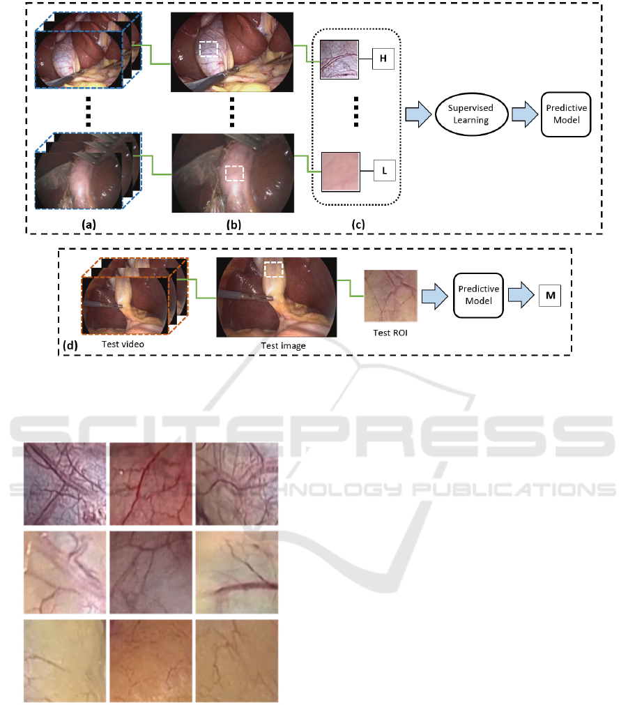
Figure 1: Graphical overview of the proposed system (see text for details). (a) Database of laparoscopic videos. (b) GB images

extracted from the videos. (c) ROIs along with annotations are provided by an expert surgeon. The ROIs are used to build a

predictive model based on supervised learning. (d) Use-case scenario: a sample ROI outlined on the GB image is classified

based on the predictive model.

Figure 2: Example image-

atches with different vascula

patterns. From top row to bottom: High-, Medium- an

Low-degree of vascularity. All patches come from differen

GB images.

Then, rectangular patches with various patterns of

vascularity were selected from the GB wall (body and

fundus areas). GB regions with specular reflection

were excluded. At this point it should be noted that

the GB may not necessarily exhibit the same vascular

pattern across its wall. There may be regions of high

vascularity separated by regions covered with fat (i.e.

low vascularity), and vice versa. Hence, a significant

step towards the assessment of the entire GB wall is

to be able to classify the vascular pattern of individual

sub-regions (patches). After experimentation with

various patch sizes, a 70 × 70 size was selected

providing a compromise between distinct pattern of

vascularity and adequate resolution to perform

assessment. Figure 2 illustrates sample image patches

with various patterns of vascularity. Note the high

inter-class color variance and the color similarity

between the middle and bottom row patches.

From the GB images, a total number of 525 image

patches was selected. The patches were classified by

a faculty surgeon based on two schemes, as this is the

first time that such a classification is examined. The

first scheme employed a 3-class classification: low-

(L), medium- (M), and high-degree (H) of

vascularity. In particular, H denotes presence of

prominent superficial vessels, L denotes absence of

vessels or extensive fat coverage, and M denotes

moderate vascularity or/and fat coverage. Second, we

employed a 2-class classification so that all patches

classified as M, were reclassified as L or H,

depending on whether they are closer to one class or

BIOIMAGING 2020 - 7th International Conference on Bioimaging

the other. An overview of the surgeon’s annotations

for the two schemes is provided in Table 1.

Table 1: Ground-truth data statistics. Number of image-

patches per class for the two classification schemes.

L M H

3-class classification

188 133 204

2-class classification

262 - 263

2.2 Classification based on

Handcrafted Features

From each image patch we extracted a rich set of

color, edge, texture, and statistical features that

describe the image on a global level (Lux and

Marques, 2013),(Vallières et al., 2015). Color and

color-edge information was based on the improved

color coherence (Pass, et al., 1996), auto color

correlogram (Huang et al., 1997), color histogram,

and color edge magnitude/direction feature vectors.

To limit the number of colors, the RGB images were

first quantized to k = 32 colors based on a k-means

algorithm applied on the training set. This method

was preferred instead of the standard uniform color

quantization process, were the RGB color space is

divided into equal-sized partitions, as it was observed

that the colors of the images distribute across a

limited region of the entire RGB space. The improved

color coherence vector takes into account the size and

locations of the regions with a particular quantized

color, whereas the auto color correlogram counts how

often a quantized color finds itself in its immediate

neighborhood. The color edge magnitude and

direction histograms were based on the gradient of

each quantized color image plane using the Sobel

gradient operator.

Image texture and edge description was based on

the Histogram of oriented gradients (HOG) (Dalal

and Triggs, 2005), Tamura features (coarseness,

contrast and directionality) (Tamura et al., 1978), and

edge histogram descriptor (Vikhar and Karde, 2016),

extracted from the intensity component of the color

image.

Moreover, we extracted various statistical

features using the radiomics feature extraction

process, applied on the quantized color image

(Vallières et al., 2015). In particular, we extracted

global features such as variance, skewness and

kurtosis as well as statistical measures using higher-

order matrix-based texture types: GLCM (gray-level

co-occurrence matrix), GLRLM (gray-level run-

length matrix), GLSZM (gray-level size zone matrix)

and NGTDM (neighborhood gray-tone difference

matrix). Note that compared to the standard

calculation of these matrices on 2D images using 8-

heignboors connectivity, in our case each color image

is considered a 3D volume and thus the texture

matrices were determined by considering 26-

connected voxels (i.e. pixels were considered to be

neighbors in all 13 directions in three dimensions).

From each texture matrix various statistical features

were extracted such as: energy, contrast, etc.

(GLCM); short run emphasis, long run emphasis, etc.

(GLRLM); small zone emphasis, large zone

emphasis, etc. (GLSZM); complexity, strength, etc.

(NGTDM).

After feature extraction from each image patch,

we performed early fusion by combining all features

resulting in a feature vector with D = 900 dimensions.

Because the number of training image-patches was

less than D, a PCA for high-dimensional data

(Bishop, 2006) was applied leading to feature vectors

with dimensionality of 165 (accounting for ≥ 95% of

the overall variability).

For the classification step we employed 3

classifiers (Bishop, 2006): Support vector machines

(SVM), k-nearest neighbors (KNN) and Naïve Bayes

(NB). For SVM we employed the Gaussian kernel;

the hyperparameters to optimize were the box

constraint and kernel scale. For KNN the

hyperparameters were the distance function

(Euclidean, cosine and city block) and the number of

nearest neighbors. NB was based on a Gaussian

kernel and the hyperparameter was the kernel window

width. For each classifier the optimization was

performed on the validation set via a grid search (10

values for each measurable hyperparameter).

2.3 CNN based Classification

The proposed CNN model is shown in Table 2.

Overall we used 3 convolutional, 3 max-pooling and

3 fully connected (FC) layers. The convolution kernel

size was 3 × 3; the convolution filters were set to 16,

32, and 64. All convolutions had stride and padding

equal to 1. Each convolution layer was followed by

Batch Normalization (Ioffe and Szegedy, 2015) and a

rectified linear unit (ReLU) activation. For max-

pooling, the stride was 2 whereas the size of the first

and the other two layers was 2 × 2 and 3 × 3,

respectively. For the three FC layers, the number of

neurons was set to 512, 256 and C (number of

classes), respectively. The first two FC layers were

followed by ReLU activation, whereas the last FC by

a softmax function, which provided the class

probabilities. To prevent overfitting, a dropout layer

with probability p = 0.2 was used after each FC layer

(except the last one) (Srivastava et al., 2014). The

Assessment of Gallbladder Wall Vascularity from Laparoscopic Images using Deep Learning

weights of the convolutional filters and FC layers

were randomly initialized from a normal distribution

with zero mean and 0.01 standard deviation, whereas

all biases were set to zero.

Table 2: The employed CNN model. BN+ReLU denotes

Batch normalization followed by ReLU. ReLU+Drop

denotes ReLU followed by dropout with probability p.

denotes the number of classes (dataset dependent).

Layer Filter size Output W×H×K

Input - 70 × 70 × 3

Conv1 3 × 3 × 16 70 × 70 × 16

BN+ReLU - 70 × 70 × 16

Max-pool1 2 × 2 35 × 35 × 16

Conv2 3 × 3 × 32 35 × 35 × 32

BN+ReLU - 35 × 35 × 32

Max-pool2 3 × 3 17 × 17 × 32

Conv3 3 × 3 × 64 17 × 17 × 64

BN+ReLU - 17 × 17 × 64

Max-pool3 3 × 3 8 × 8 × 64

FC1 - 512

ReLU+Drop - 512

FC2 - 256

ReLU+Drop - 256

FC3 - C

Softmax - C

During training we adopted a batch size of 35 and

the Adam optimization with default parameters

(Kingma and Ba, 2014). The loss function was based

on the categorical cross-entropy:







,

log









(1)

where j ∊ {1,…,C} is the class index, y

i,j

∊ {0,1}

is the ground truth corresponding to class j and image

i, and φ(·) denotes the softmax output for the

activations of the FC3 layer. To reduce overfitting, an

regularization term (weight decay) with λ = 1e-4

was added to the loss function.

The model was trained either for 40 epochs or

until the loss on the validation set was larger than the

previously smallest loss for 5 evaluations. The

evaluation was performed every 10 iterations. The

initial learning rate was 0.001, which was dropped by

a factor of 0.1 after every 8 epochs. To increase the

dataset size and improve generalization of the model,

data augmentation was performed: horizontal flip,

vertical flip and rotation by ±30

and ±60

3 EXPERIMENTAL RESULTS

The image patch dataset was randomly split into

training (60%), validation (20%) and test set (20%),

based on a 5-fold cross validation. Specifically, the

image patches were randomly split into five parts of

equal size with the constraint to preserve the

frequency of each class among the folds. The

frequency of each class was also preserved among the

three sets in each fold. Each of the five folds was

selected as test-set and the other ones for training and

validation. The performance of the aforementioned

approaches was evaluated in terms of the following

metrics:

Acc = (TP + TN)/(P + N) (2)

Pre = TP/(TP + FP) (3)

Rec = TP/(TP + FN) (4)

F1 = 2 × Pre × Rec/(Pre + Rec) (5)

where Acc, Pre, Rec, F1 denote: Accuracy,

Precision, Recall, and F1-score, respectively; TP, TN,

FP, FN, P, N denote: true positives, true negatives,

false positives, false negatives, positives and

negatives, respectively. In addition, we computed the

area under curve (AUC) from the receiver operating

characteristic (ROC) plot (i.e. true positive rate =

TP/P vs. false positive rate = FP/N). The results are

presented as mean values across the 5 folds, unless

otherwise stated.

Table 3 shows the performance of the four

methods for the 2-class classification problem (i.e. L

vs. H). The performance metrics of all methods are ≥

91%. The CNN model achieves the best performance

across all metrics; its accuracy is 98% and a similar

value is observed for the mean Precision, Recall and

F1-score of the two classes (Table 4). SVM is the

second best method with ~2% lower performance.

KNN is ranked third (~94.4% mean performance) and

NB fourth (~92.2% mean performance). It is worth

noting that for all methods the Recall for the H class

is higher than that of the L class, which means that

high vascularity images are discriminated slightly

better. The Precision of the CNN for the two classes

is similar (~98%), so the model generates similar

false positives. For the other methods, the Precision

between the classes is mixed. Figure 3 shows the

normalized confusion matrices of the four methods.

The matrices were normalized after summation of the

raw confusion matrices of the test-folds. From NB to

CNN the performance rises with increasing on Recall

and decreasing on misclassification (false positives).

BIOIMAGING 2020 - 7th International Conference on Bioimaging

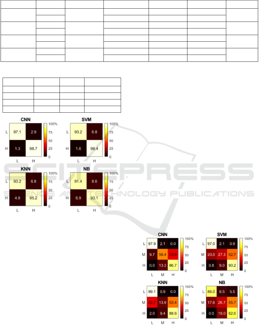
Table 3: Performance comparison for 2-class classification.

Table 4: Mean performance comparison for 2 classes.

Method Pre (%) Rec (%) F1 (%)

CNN 98.0 97.9 98.0

SVM 96.5 95.8 96.1

KNN 94.4 94.2 94.2

NB 92.3 92.2 92.2

Figure 3: Color-coded confusion matrices for 2-class

classification. The X and Y-axis represent predicted and

ground truth labels, respectively.

Table 5 shows the methods’ performance for the

ranking of the methods with respect to their

performance is the same as that in 2-class

classification (1

CNN, 2

SVM, 3

KNN and 4

NB), although in overall the methods’ performance is

lower, as expected. Specifically, the accuracy of the

CNN is 83.1% whereas the mean Precision, Recall

and F1-score of the three classes is 81.5%, 80.3% and

80.4%, respectively (Table 6).

From Table 5 it is observed that the Recall of the

L class is higher than that of the other two classes,

denoting better classification for the L class. The

same result is also valid for the Precision of the L

class, implying that misclassification of the other two

classes as L is lower. Moreover, for the L and H

classes the Recall is higher than Precision, denoting

that the methods generate less false negatives

compared to false positives. Among the three classes,

the best performance is yielded for the L class and the

worst for the M class. For the CNN model, the F1-

scores of the three classes are: 95.7% (L), 83.0% (H)

and 62.7% (M). It is worth noting that this

performance ranking is the same in all methods.

However, the performance of the SVM, KNN and NB

is much lower than CNN’s.

For the CNN model and the L class, it can be

noticed that compared to 2-class classification (Table

3), in 3-class classification (Table 5), the Precision

and F1 are only 4.6% and 2% lower respectively,

whereas the Recall is 0.8% higher. However, the

performance of the H class deteriorates considerably

(≥ 12%). Hence, it seems that the addition of the M

class has a negative impact on the classification of the

H class, mostly because samples between these two

classes are misclassified as one another. This may

also be noticed from Figure 4 that shows the

normalized confusion matrices. It is observed that: (a)

the CNN yields no confusion between L and H,

whereas in the other methods there is a slight

confusion, (b) the H class is more confused as M than

what the L class is, (c) the M class is mostly confused

Figure 4: Color-coded confusion matrices for 3-class

classification. The X and Y-axis represent predicted and

ground truth labels, respectively.

Method Class Acc (%) Pre (%) Rec (%) F1 (%) AUC

CNN

98.0

98.2 97.1 97.7

0.996

H 97.9 98.7 98.3

SVM

96.2

97.8 93.2 95.4

0.991

H 95.1 98.4 96.7

KNN

94.4

93.7 93.2 93.4

0.969

H 95.0 95.2 95.1

92.4

91.0 91.4 91.1

0.977

H 93.7 93.1 93.3

Assessment of Gallbladder Wall Vascularity from Laparoscopic Images using Deep Learning

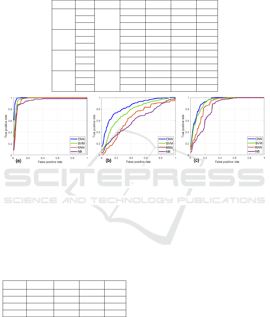
Table 5: Performance comparison for 3-class classification.

Method Class Acc (%) Pre (%) Rec (%) F1 (%) AUC

CNN

83.1

93.6 97.9 95.7

0.992

M 71.0 56.4 62.7

0.843

H 79.8 86.7 83.0

0.929

SVM

76.8

86.7 97.0 91.6

0.977

M 67.0 27.3 36.9

0.759

H 72.2 90.2 80.0

0.916

KNN

73.6

79.9 99.1 88.5

0.965

M 46.9 13.9 21.3

0.663

H 72.0 88.6 79.5

0.883

69.5

87.3 86.0 86.4

0.947

M 38.5 26.7 31.1

0.605

H 67.3 82.0 73.6

0.845

Figure 5: The ROC curves for the: (a) L, (b) M and (c) H classes, respectively.

as H and this confusion is greater than all other

confusions, and (d) the confusion of the M class as H

is more than the confusion of H as M. Overall, CNN

outputs the fewest misclassifications across the three

classes.

Tables 5 and 6 also report the classes’ and class-

average AUC values, respectively. The mean ROC

curves for every class and method are depicted in

Figure 5. The CNN model yields the highest AUC

across all classes: 0.992 (L), 0.843 (M) and 0.929 (H),

something that may be also concluded from the ROC

curves.

Table 6: Mean performance comparison for 3 classes.

Method Pre (%) Rec (%) F1 (%)

AUC

CNN 81.5 80.3 80.4

0.921

SVM 75.3 71.5 69.5

0.884

KNN 66.3 67.2 63.1

0.837

NB 64.4 64.9 63.7

0.799

4 CONCLUSIONS

In this paper we present a novel idea for visual

assessment of the GB wall vascularity from

intraoperative LC images, based on machine learning.

To the best of our knowledge, the research work

presented in this paper is the first one that attempts to

investigate this application field. As described in the

Introduction, the vascular pattern of the GB wall

provides some clues about the GB condition, the

operation complexity, potentially need of extra

resources (e.g. advanced surgical skills) and generally

a means to characterize the operation. The

classification of the vascular pattern was based on

two alternative evaluations provided by an

experienced surgeon (2-class classification and 3-

class classification), as there is no established

consensus about the most appropriate vascularity

grading scheme from laparoscopic images. Our

results lead to the following conclusions.

First, the CNN model outperforms all other

methods both in 2-class and 3-class classification

(e.g. by ≥ 1.8% and ≥ 6.3% in accuracy, respectively).

Second, for all methods the best performance is

achieved in 2-class classification. Third, in 2-class

and 3-class classification, the CNN model yields a

very high performance for the L class (Pre ≥ 93.6%

and Rec ≥ 97.1%). Fourth, for the H class the

performance is very high in 2-class classification (Pre

= 97.9% and Rec = 98.7%), but lower in 3-class

BIOIMAGING 2020 - 7th International Conference on Bioimaging

classification (Pre = 79.8% and Rec = 86.7%). Fifth,

the inclusion of the M class mostly deteriorates the

performance of the H classification (e.g. for CNN:

13.3% confusion). Moreover, the M class is mostly

confused as H (33.9% for CNN), something that is

observed for all methods. Hence, the M class was the

most difficult one to recognize. A quantitative

measure of independent reviewers’ agreement on the

annotation of the M class would help evaluating the

difficulty of this task, or even whether the 3-class

classification scheme is indeed appropriate for our

application. In the future we aim to elaborate further

on this issue.

Given that this study investigates a novel

application in the area of computer assisted surgery,

there are still open issues for further research. First,

the results in this study are based on the ground truth

assessment

provided by a single expert. The

recruitment of additional experts is essential in order

to evaluate their level of agreement and most

importantly to establish the most appropriate

vascularity annotation scheme. Moreover, we aim to

expand our dataset by including more images from

additional LC operations. Second, the results are

based on classification of patches extracted from GB

images. Hence, it is important to extend the CNN

model to predict the vascular pattern of the entire GB

region in the laparoscopic image. A potential solution

would be to sequentially extract patches from a user-

specified GB region and then aggregate the CNN’s

patch predictions. The investigation of more

advanced CNN models, alternative loss functions to

penalize misclassifications of extreme classes, and

color preprocessing techniques for visual

enhancement of the GB wall vessels, are also major

topics of interest for future research work.

ACKNOWLEDGEMENTS

The author thanks Special Account for Research

Grants and National and Kapodistrian University of

Athens for funding to attend the meeting.

REFERENCES

Bishop, C.M., 2006. Pattern recognition and machine

learning. New York: Springer-Verlag New York, Inc.

Dalal, N. and Triggs, B., 2005. Histograms of Oriented

Gradients for Human Detection, In IEEE Computer

Society Conference on Computer Vision and Pattern

Recognition (CVPR’05), pp. 886–893.

Huang J. et al., 1997. Image indexing using color

correlograms, In Proceedings of IEEE Computer

Society Conference on Computer Vision and Pattern

Recognition. IEEE Comput. Soc, pp. 762–768.

Ioffe, S. and Szegedy, C., 2015. Batch Normalization:

accelerating deep network training by reducing internal

covariate shift, In Proceedings of the 32nd

International Conference on International Conference

on Machine Learning (ICML ’15), pp. 448–456.

Jin, A. et al., 2018. Tool detection and operative skill

assessment in surgical videos using region-based

convolutional neural networks, In IEEE Winter

Conference on Applications of Computer Vision

(WACV). Lake Tahoe, NV, USA, pp. 691–699.

Jin, Y. et al., 2019. Multi-task recurrent convolutional

network with correlation loss for surgical video

analysis. arXiv preprint. Available at:

http://arxiv.org/abs/1907.06099.

Kingma, D.P. and Ba, J, 2014. Adam: a method for

stochastic optimization. arXiv preprint. Available at:

http://arxiv.org/abs/1412.6980.

Loukas, C. et al., 2016. Shot boundary detection in

endoscopic surgery videos using a variational Bayesian

framework, International Journal of Computer Assisted

Radiology and Surgery, 11(11), pp. 1937–1949.

Loukas, C. et al., 2018. Keyframe extraction from

laparoscopic videos based on visual saliency detection,

Computer Methods and Programs in Biomedicine, 165,

pp. 13–23.

Loukas, C., 2018. Video content analysis of surgical

procedures, Surgical Endoscopy, 32(2), pp. 553–568.

Loukas, C. and Georgiou, E., 2013. Surgical workflow

analysis with Gaussian mixture multivariate

autoregressive (GMMAR) models: a simulation study,

Computer Aided Surgery, 18(3–4), pp. 47–62.

Loukas, C. and Georgiou, E., 2015. Smoke detection in

endoscopic surgery videos: a first step towards retrieval

of semantic events, International Journal of Medical

Robotics and Computer Assisted Surgery, 11(1), pp.

80–94.

Loukas, C. et al., 2011. The contribution of simulation

training in enhancing key components of laparoscopic

competence, The American Surgeon, 77(6), pp. 708-

715.

Lux, M. and Marques, O., 2013. Visual information

retrieval using Java and LIRE, Synthesis Lectures on

Information Concepts, Retrieval, and Services. Edited

by G. Marchionini. Morgan & Claypool.

Pass, G. et al., 1996. Comparing images using color

coherence vectors, In

Proceedings of the fourth ACM

international conference on Multimedia-

MULTIMEDIA ’96. New York, New York, USA: ACM

Press, pp. 65–73.

Petscharnig, S and Schöffmann, K., 2018. Binary

convolutional neural network features off-the-shelf for

image to video linking in endoscopic multimedia

databases, Multimedia Tools and Applications, 77(21),

pp. 28817–28842.

Assessment of Gallbladder Wall Vascularity from Laparoscopic Images using Deep Learning

Pontarelli, E.M. et al., 2019. Regional cost analysis for

laparoscopic cholecystectomy, Surgical Endoscopy,

33(7), pp. 2339–2344.

Srivastava, N. et al., 2014. Dropout: a simple way to prevent

neural networks from overfitting, Journal of Machine

Learning Research, 15(1), pp. 1929–1958.

Tamura, H., Mori, S. and Yamawaki, T., 1978. Textural

features corresponding to visual perception, IEEE

Transactions on Systems, Man, and Cybernetics, 8(6),

pp. 460–473.

Twinanda, A.P. et al., 2015. Classification approach for

automatic laparoscopic video database organization,

International Journal of Computer Assisted Radiology

and Surgery, 10(9), pp. 1449–1460.

Twinanda, A.P. et al., 2017. EndoNet: A deep architecture

for recognition tasks on laparoscopic videos, IEEE

Transactions on Medical Imaging, 36(1), pp. 86–97.

Twinanda, A.P. et al., 2019. RSDNet: learning to predict

remaining surgery duration from laparoscopic videos

without manual annotations, IEEE Transactions on

Medical Imaging, 38(4), pp. 1069–1078.

Vallières, M. et al., 2015. A radiomics model from joint

FDG-PET and MRI texture features for the prediction

of lung metastases in soft-tissue sarcomas of the

extremities, Physics in Medicine and Biology, 60(14),

pp. 5471–5496.

Vikhar, P. and Karde, P., 2016. Improved CBIR system

using Edge Histogram Descriptor (EHD) and Support

Vector Machine (SVM), In International Conference

on ICT in Business Industry & Government (ICTBIG).

IEEE, pp. 1–5.

BIOIMAGING 2020 - 7th International Conference on Bioimaging