
Visualizing Syscalls using Self-organizing Maps for System Intrusion
Detection
Max Landauer
1
, Florian Skopik
1
, Markus Wurzenberger
1
, Wolfgang Hotwagner
1
and Andreas Rauber
2
1
Austrian Institute of Technology, Center for Digital Safety & Security, Vienna, Austria
2
Vienna University of Technology, Institute of Information Systems Engineering, Vienna, Austria
Keywords:
Anomaly Detection, Self-organizing Maps, Syscall Logs, Visualization.
Abstract:
Monitoring syscall logs provides a detailed view on almost all processes running on a system. Existing ap-
proaches therefore analyze sequences of executed syscall types for system behavior modeling and anomaly
detection in cyber security. However, failures and attacks that do not manifest themselves as type sequences
violations remain undetected. In this paper we therefore propose to incorporate syscall parameter values with
the objective of enriching analysis and detection with execution context information. Our approach thereby
first selects and encodes syscall log parameters and then visualizes the resulting high-dimensional data using
self-organizing maps to enable complex analysis. We thereby display syscall occurrence frequencies and tran-
sitions of consecutively executed syscalls. We employ a sliding window approach to detect changes of the
system behavior as anomalies in the SOM mappings. In addition, we use SOMs to cluster aggregated syscall
data for classification of normal and anomalous system behavior states. Finally, we validate our approach on
a real syscall data set collected from an Apache web server. Our experiments show that all injected attacks are
represented as changes in the SOMs, thus enabling visual or semi-automatic anomaly detection.
1 INTRODUCTION
Modern computer systems are almost always at risk
of being compromised by adversaries. In particular,
systems that are connected to a network are subject to
malware infections or intrusions executed with the use
of sophisticated tools. As a countermeasure, cyber
security employs monitoring techniques that continu-
ously check applications and processes for signatures
that indicate malicious activities.
However, signature based detection approaches
that rely on predefined patterns are unable to detect
attacks that have never been observed before. As a
solution, anomaly detection enables the disclosure of
previously unknown attacks and failures by recogniz-
ing repeating patterns as normal system behavior and
reporting any deviations from the learned models as
potential threats (Chandola et al., 2009).
Adequate and correctly configured data sources
are essential for monitoring system behavior in suf-
ficient detail so that manifestations of normal actions
as well as attacks are visible. Other than most ap-
proaches that analyze network traffic for anomaly de-
tection, the focus of our work lies on system log
data, because these logs are semantically more ex-
pressive and contain verbose information about al-
most all events that take place on a system, not only
what is communicated with other machines (Creech
and Hu, 2014; Liu et al., 2011).
Log messages are frequently collected, processed
and analyzed in Security Information and Event Man-
agement (SIEM) systems (Kavanagh et al., 2018).
These systems usually provide interactive dashboards
that visualize monitored log events in real-time. Un-
fortunately, these visualizations are usually limited
to simple charts that display the frequencies of log
events relative to each other, or graphs containing
time-series of event occurrences. We argue that
such simple visualizations do not adequately exploit
the potential of representing information contained
within log events such as syscalls.
Syscalls (system calls) are a type of log data avail-
able in almost all operating systems. Because of their
verbosity and fine-grained view on the executed com-
mands, syscalls are frequently used for forensic sys-
tem analysis after attacks. Shifting to a more proac-
tive analysis, continuously monitoring syscalls using
enables automatic anomaly detection and shortens the
Landauer, M., Skopik, F., Wurzenberger, M., Hotwagner, W. and Rauber, A.
Visualizing Syscalls using Self-organizing Maps for System Intrusion Detection.
DOI: 10.5220/0008918703490360
In Proceedings of the 6th International Conference on Information Systems Security and Privacy (ICISSP 2020), pages 349-360
ISBN: 978-989-758-399-5; ISSN: 2184-4356
Copyright
c
2022 by SCITEPRESS – Science and Technology Publications, Lda. All rights reserved
349

reaction time after incidents, while at the same time
reducing the required domain knowledge and time
spent with manual analysis.
Existing works that pursue anomaly detection on
syscalls often focus on the sequences of syscall types
alone, i.e., they only consider a single value from the
syscall log lines. However, sophisticated attacks are
designed to resemble legitimate syscall execution se-
quences and thus evade such detection mechanisms
(Shu et al., 2015). There is thus a need for anomaly
detection techniques that are able to incorporate the
execution context in the analysis process. We propose
to use argument and return values as well as user and
process information to enrich behavior models de-
rived from syscall sequences. It is non-trivial to pre-
pare this high-dimensional data in a way that supports
visual review for manual and semi-automatic analysis
of syscall sequences and occurrence frequencies. We
solve this issue by employing self-organizing maps
(SOM) to group and position the syscall log data in a
two-dimensional space for visualization.
We summarize our contributions as follows:
• An approach for visualizing system behavior
through syscall logs using self-organizing maps,
• enabled by a method for selecting and encoding
relevant features,
• with the purpose of manual or semi-automatic
anomaly detection.
The paper is structured as follows. Section 2 re-
views existing approaches for syscall anomaly detec-
tion and visualization. Section 3 provides general in-
formation on syscalls and discusses log data prepro-
cessing. Basics on SOM visualizations and advanced
visualizations of system behavior are outlined in Sect.
4 and Sect. 5 respectively. Our experiments and the
resulting plots are presented in Sect. 6 and discussed
in Sect. 7. Finally, Sect. 8 concludes the paper.
2 RELATED WORK
Monitoring syscalls for cyber security has been an
ongoing research for many years. One of the earli-
est popular approaches was proposed by Forrest et al.
(Forrest et al., 1996), who used a sliding window to
learn a model of normal system behavior from syscall
traces that comprises all observed sequences. After
the learning phase, any appearing sequence not repre-
sented by that model is considered an anomaly.
One critical issue with this and similar succeed-
ing approaches is that they only consider the type of
syscall, but omit all other parameters. This results
in simpler models, but also impairs the capability of
detecting attacks, in particular when attackers design
their attacks to resemble benign syscall sequences. In
order to alleviate this issue and improve the ability
to detect such stealthy or mimicry attacks (Shu et al.,
2015), modern approaches attempt to include the con-
text of syscall execution in their analyses.
To address this issue, Abed et al. (Abed et al.,
2015) include execution context about closely occur-
ring syscalls by computing their frequencies in slid-
ing time windows. Similarly, Yoon et al. (Yoon et al.,
2017) use frequency distributions to cluster syscalls
into profiles. In addition to clustering, Shu et al. (Shu
et al., 2015) use syscall occurrence frequencies within
clusters as well as their co-occurrences relevant for
the detection of anomalies.
In many works, neural networks are employed,
because of their prominent ability to detect reoccur-
ring patterns in sequences. For example, Kim et al.
(Kim et al., 2016) make use of ensembles of a par-
ticular type of recurrent neural network named Long
Short-Term Memory (LSTM) network, which is able
to compute the probability distributions of syscalls
that follow a given sequence. Creech and Hu (Creech
and Hu, 2014) first identify common sequences of
syscalls as words and then use these words as an in-
put to a fast-learning neural network type called Ex-
treme Learning Machine in order to detect phrases,
i.e., common sequences of these words.
Our approach employs self-organizing maps,
which also belong to the family of neural networks,
but their application differs greatly compared to ex-
isting work. Rather than explicitly learning the se-
quences of appearing syscalls, we use SOMs to group
and place them in an euclidean space, so that the tran-
sitions between them become visually apparent. In
addition, our approach incorporates syscall parame-
ters to enable context-aware analysis. Also Liu et al.
(Liu et al., 2011) take syscall arguments into consider-
ation, but use them to form semantic units, i.e., groups
that describe specific aspects of program behavior.
Providing visualizations that make syscall se-
quences intuitively understandable is non-trivial.
Saxe et al. (Saxe et al., 2012) group and visualize
syscall sequences of malware. Their approach relies
on a similarity matrix of syscall sequences that is used
to arrange malware on a grid so that clusters of related
malware emerge. In addition, they provide a method
for visual comparison of malware by rendering their
subsequences as sequential colored blocks.
Other approaches that support syscall visualiza-
tions are usually limited to control-flow graphs gen-
erated by linking the learned benign sequences (Es-
kin et al., 2001). However, these graphs do not take
context information into account, and would require
ICISSP 2020 - 6th International Conference on Information Systems Security and Privacy
350

type=SYSCALL msg=audit(1551210435.995:23194): arch=c000003e syscall=1 success=yes exit=19 a0=d
a1=42 a2=180 a3=0 items=0 ppid=2249 pid=2253 auid=0 uid=33 gid=33 euid=33 suid=33 fsuid=33 egid=33
sgid=33 fsgid=33 tty=(none) ses=2 comm=”apache2” exe=”/usr/sbin/apache2” key=(null)
Figure 1: Sample syscall log line of an Apache process.
Table 1: One-hot encoded sample syscall log line.
syscall 1 syscall 2 syscall 257 success yes success no exit -2 exit 0 exit 19 exit * ...
1 0 0 1 0 0 0 1 0 ...
copies of nodes when syscalls appear with different
parameters, leading to a high complexity. SOMs
alleviate this problem by automatically placing the
syscall instances according to the similarity of their
parameters, thereby effectively clustering the data.
Girardin and Brodbeck (Girardin and Brodbeck,
1998) experiment with approaches to visualize net-
work data, including SOMs. However, their approach
focuses only on labeling the SOM for static analysis
or real-time monitoring. While we also discuss la-
beling for overview, our approach visualizes node hit
frequencies and node transitions in the SOM and ad-
ditionally makes use of sliding time windows to detect
changes of consecutively generated SOMs.
3 SYSCALLS
Syscall log data contains a mixture of categorical
(e.g., syscall types) and textual (e.g., path names)
values and is thus not directly applicable for train-
ing a model using machine learning without appropri-
ate preprocessing. This section therefore investigates
characteristics of syscalls, including the collection of
syscall log data and properties of the data that enable
the generation of a system behavior model.
3.1 Characteristics
Syscalls are used by almost all applications for com-
municating with and requesting services from the
kernel of the operating system that the applications
run on. Employing syscalls as an intermediary is
thereby a necessary step to provide controlled access
to security-critical system components. There usu-
ally exist hundreds of different available system calls
in most modern operating systems, some of the most
common being open, read, or exec (Mandal, 2018).
In busy systems, service requests to the kernel are
frequent, which generates long sequences of syscalls.
Theoretically, the possible amount of combinations of
consecutive syscall types is immense; however, inves-
tigating syscalls shows that occurring syscall subse-
quences are highly regular and contain chains of re-
peating patterns. The reason for this is that applica-
tions execute the same machine code over and over,
thereby generating similar syscall sequences multiple
times. Moreover, the steps necessary for carrying out
particular tasks are usually not subject to change over
time, but are relatively constant (Forrest et al., 1996).
Therefore, mining frequently occurring sequences al-
lows to generate normal system behavior models.
Parameters of syscalls on the other hand are more
variable than syscall types and usually depend on the
elapsed time, user input, other processes, or the sys-
tem environment. While this makes them consider-
ably more difficult to analyze than just the sequences
of syscall types alone, they express the purpose of
the syscall in a more fine-grained detail and are thus
able to reveal information on the context in which
the syscall is executed (Liu et al., 2011). When this
context is expanded to not just one, but sequences of
syscalls, conclusions on the current state of the system
with respect to all its active processes can be drawn.
Incorporating context is a key aspect for utiliz-
ing syscalls for security, since any attacks or exploits
are highly likely to manipulate or spawn processes
and thus manifest themselves within the syscall logs.
Thereby, a single syscall instance alone may not nec-
essarily be reasonably recognizable as part of a mali-
cious process; but rather one or multiple syscalls that
are executed within a specific context may be indica-
tors that the system has been compromised.
Figure 1 shows a sample syscall log line from
an Apache server. Since the syntax of the lines are
known and only consist of key-value pairs, a parser
is able to extract all relevant parameters from such a
syscall log line, including the time stamp, CPU ar-
chitecture (arch), syscall type, return values (success,
exit), arguments (a0 to a3), user information (uid,
gid), process information (pid, comm, exe), and sev-
eral more. In addition, a number of PATH records
may follow each syscall (indicated by items). It is
usually not feasible and reasonable to include all pa-
rameters when generating self-organizing maps. The
following section explains the difficulties and outlines
a method for selecting suitable parameters.
Visualizing Syscalls using Self-organizing Maps for System Intrusion Detection
351

3.2 Feature Selection
One important observation from the sample syscall
log line shown in Fig. 1 is that all parameters (ex-
cept the timestamp) should be treated as categorical
variables, since it is not possible to establish proper
ordinal relationships between the values, even though
some of them are numeric. For example, syscall type
1 (write) is in no way closer related to syscall type 2
(open) than to syscall type 257 (openat).
One possibility to enforce correct handling of cat-
egorical features is to apply one-hot encoding (Har-
ris and Harris, 2007) to the extracted parameters. For
this, it is first necessary to identify all unique values of
a parameter to be encoded. In the second step, the pa-
rameter is replaced with a range of parameters, where
each of them specifies whether the respective value is
present in the syscall log line (1) or not (0). Table
1 shows some encoded parameters of the sample log
line from Fig. 1. Thereby, the original name of the
parameter is specified before the underline character,
followed by the value. In this sample, three syscall
types (1, 2, 257) are present in the data, and accord-
ingly three parameter-value pairs exist, of which the
first one is set to 1 and all others to 0 corresponding
to the syscall type 1 in the sample log line. This is
carried out analogously for all other parameters. Note
that for each set of parameter-value pairs, only a sin-
gle 1 is allowed, since each parameter exists only once
in each log line.
Unfortunately, parameters that contain only or
high amounts of unique values result in a massive
enlargement of the resulting feature vector, but only
contribute little or nothing to the ability of grouping
the syscall observations, because the values are al-
most always 0 for each observation. Simply omitting
such parameters is not recommended, because there
may be one or few values that occur more often than
others, which can be relevant feature for clustering.
For example, half of all syscall log lines could have
argument a3=0, while all others have unique values
for this parameter. We suggest to group all values
with insufficiently high occurrence frequency in a sin-
gle wildcard-bucket, e.g., all values of a feature that
occur in less than 5% of all rows. This ensures that
frequently occurring values relevant for clustering re-
main in the data, while at the same time vector di-
mension is kept within reasonable bounds. Table 1
shows this idea applied to the parameter exit, where
all exit values other than -2, 0, 19 are allocated to
exit *. Syscalls in this vector format are suitable for
training a SOM. The SOM training process is outlined
in the following section.
4 SELF-ORGANIZING MAPS
This section covers the basics of self-organizing maps
(Kohonen, 1982). We also mention differences to typ-
ical SOM applications and the role of SOMs in our
approach.
4.1 Overview
A self-organizing map (SOM) is a type of neural
network that supports unsupervised learning. The
main goal is to visually represent high-dimensional
input data within a low-dimensional (typically two-
dimensional) space while maintaining topological
properties as closely as possible. This is achieved by
assimilating inherent structures of the input data by a
set of nodes that are usually arranged within a rectan-
gular or hexagonal grid of predefined size. Displaying
the trained grid in a two-dimensional space is a useful
tool for visualization.
The training procedure is as follows: a weight
vector of the same dimension as the input data with
initially random values is assigned to each node of
the grid. The input vector of each syscall instance is
then iteratively presented to the network, which learns
structures of the input data by adjusting the weight
vectors accordingly. Other than most existing neural
networks, SOMs pursue competitive learning, mean-
ing that for each syscall observation, the best match-
ing unit (BMU) is selected by computing the mini-
mal distance between the input vector and all of the
weight vectors. Typical selections for the distance
function are the Euclidean distance for continuous
data and the Manhattan distance for binary or cate-
gorical data. The weight vector of the best matching
unit is then modified to resemble the currently pro-
cessed input vector more closely using a predefined
learning rate. In addition, all neighboring nodes of
the best matching unit are modified analogously, but
to a lesser degree. This is carried out iteratively for
all syscall observations in the input data and typically
repeated several hundred times, until the weights of
the grid reach stability (Kohonen, 1982).
As explained in Sect. 3.2, the approach proposed
in this paper makes use of one-hot encoded input
data in order to handle categorical values correctly.
This binary data influences the typical outcome of the
SOM: it is less common that input vectors fit “in-
between” frequently hit nodes, i.e., relative to the size
of the grid, only a small amount of nodes are se-
lected as best matching units. This leads to the forma-
tion of relatively clear boundaries between the nodes,
which is not usual when SOMs are trained with con-
tinuous ratio scales that typically result in smooth and
ICISSP 2020 - 6th International Conference on Information Systems Security and Privacy
352

gradually changing structures. Accordingly, the SOM
functions more like a clustering algorithm that groups
similar syscall log lines in the same nodes, but has the
advantage to automatically determine the importance
of each feature for each node and additionally main-
tains an overall topology useful for visualization.
4.2 Node Labels
Node labels improve the expressiveness and simplify
interpretation of SOMs, because they represent the
most important syscall properties and display which
features are shared or differ between neighboring
nodes. We therefore print the names of the most rele-
vant features onto each node.
We mentioned that the binary input data affects
the overall distribution of the nodes, but it also has
an effect on their labels. Other than for contin-
uous data where the feature weights of each node
are not bounded, the weights in our setup lie within
the range [0, 1]. Given that the input vectors are
high-dimensional, it is not unusual that several fea-
ture weights computed at some nodes reach the max-
imum value of 1, meaning that the corresponding
features are all equally important for describing the
node, making automatic selection difficult. In addi-
tion, since these weights are computed solely using
the vector instances that are mapped to the respec-
tive nodes or their neighborhood as outlined in Sect.
4.1, they may not necessarily be appropriate to de-
scribe the node with respect to rest of the grid or the
other data instances. For example, a feature that is
1 in every instance of the whole data set yields the
same weight of 1 at every node as another feature that
is 1 only in the instances mapped to a specific node,
and 0 in all other instances. However, the latter fea-
ture describes what makes that specific node different
from the rest of the grid and is thus an arguably more
informative label for the node.
We propose to alleviate this issue as follows. For
each node n ∈ N, compute the relative amount of ones
separately for every feature n
1
, n
2
, ..., n
N
considering
all instances mapped to that node, i.e., r
1
, r
2
, ..., r
N
with r
i
=
∑
n
i
÷
|
n
|
, where
|
n
|
is the number of in-
stances mapped to n. Then compute the relative
amount of ones for every feature considering all in-
stances that are not mapped to that node, i.e., use the
rest of the instances from the whole data set m = N \n
to compute s
1
, s
2
, ..., s
N
by s
i
=
∑
m
i
÷
|
m
|
. Finally,
compute the vector w = r−s that is higher for features
that are present many times in the node instances, but
rare in the data set. We see this value as a weight that
indicates the most interesting features that distinguish
the nodes and thus use it to select the labels.
Note that it is also possible to approach this issue
conversely by considering the absence of a feature as
an appropriate descriptor for a node. This is carried
out in the same manner, but computing the relative
amounts of zeros present in the data instances mapped
on the node and the data set respectively. However, it
is less intuitive to comprehend this kind of labeling
and it was therefore omitted.
We also want to point out that due to the fact that
the one-hot encoded data of one specific syscall log
parameter always must only have a single 1 in all
the features belonging to that parameter, it is unlikely
that more than one feature corresponding to the same
syscall log parameter are within the set of highest-
weighted features. Considering the sample shown in
Table 1, this means that it is unlikely that both fea-
tures syscall 1 and syscall 2 are within the top ranked
features, but rather a mixture of different parameters.
5 SYSTEM BEHAVIOR ANALYSIS
The previous section explained relevant properties of
SOMs with respect to binary input data that is derived
from syscall log lines. In this section we build upon
these insights and propose concepts for deriving sys-
tem behavior from the SOM.
5.1 Frequency Analysis
After training the SOM is completed, it is possible to
map every syscall feature vector from the input data
set to the node that yields the lowest distance to that
input vector, analogously to the learning process de-
scribed in Sect. 4.1. Visualizing these hit frequen-
cies of all nodes results in a so-called hit histogram
that displays the distribution of syscall execution fre-
quency across the nodes. The hit distribution is rele-
vant for system behavior analysis, because in steady
systems the relative amounts of occurrences of all
syscall types are normally expected to be quite sta-
ble within identically sized time windows, or follow
periodic behavior.
We use logarithmic scaling for visualizing hit dis-
tributions. The reason for this is that in almost all real
systems, syscall frequency distributions are highly
unbalanced, making it difficult to recognize devia-
tions on low-frequency nodes. An example of a hit
histogram is given in the following section.
5.2 Sequence Mining
Hit histograms represent a static unordered view on
the syscalls appearing within a time window and thus
Visualizing Syscalls using Self-organizing Maps for System Intrusion Detection
353

syscall_93
success_yes
exit_361
syscall_5
success_yes
exit_361
syscall_3
success_yes
exit_361
syscall_91
success_yes
exit_361
syscall_85
success_yes
exit_361
syscall_82
success_yes
exit_361
success_no
exit_−2
syscall_146
syscall_146
success_yes
exit_361
syscall_4
success_yes
exit_361
Freq (log)
0.0
0.5
1.0
1.5
2.0
Figure 2: SOM of three sample processes (orange and yel-
low loops of arrows), including one anomaly (red arrows).
lack the ability to represent the sequences of syscalls.
Our approach therefore connects nodes that are con-
secutively hit with arrows that point from each node
to the subsequently hit node. When the same node is
hit twice in a row, we insert a circular arrow pointing
from the node to itself. We superimpose all arrows on
the hit histogram and color the arrows according to
the number of times this connection is present in the
data, where yellow indicates a high number of transi-
tions, orange indicates a moderate number of transi-
tions, and red indicates a low number of transitions.
Again, logarithmic scaling is applied.
Figure 2 shows a demonstration of the mentioned
concepts on sample data. The data used for this vi-
sualization captures the three processes P1, P2, and
P3 that continuously execute the following types of
syscalls: P1 executes 93-91-82-93-91-82-..., P2 exe-
cutes 3-4-146-3-4-146-..., and P3 executes 3-5-5-85-
3-5-5-85-... over a long period of time, where each
number corresponds to a particular syscall operation,
such as opening a file or executing a task. Several
conclusions can be drawn from the plot: First, all
processes are correctly depicted. The smaller orange
loop of arrows in the bottom right corner corresponds
to P1, the yellow loop of arrows corresponds to P2,
and the larger orange loop of arrows in the bottom
corresponds to P3. It is easy to distinguish the pro-
cesses by observing the node labels where the syscall
type is placed as the most relevant characteristic of
most nodes, because it is the most diverse feature in
the data. Second, P2 contains an anomaly that mani-
fests itself as a syscall of type 146 that returns an un-
successful exit code -2 instead of the successful exit
code 361. Such an anomaly could not be detected by
a system behavior modeling approach that only takes
syscall type numbers into account. Accordingly, the
labels show that the parameters are higher weighted
than the syscall type. Third, the hit histogram shows
that the node of brightest color corresponds to syscall
type 3, meaning that it is most frequently hit. This
is reasonable, because both P2 and P3 make use of
syscall type 3. Fourth, the arrow colors show that the
yellow loop of transitions corresponding to P2 is the
most active of all processes, and that the anomalous
syscall was only executed very infrequently as indi-
cated by the red arrows.
Note that processes usually overlap each other and
are often executed in parallel. This causes that the se-
quences of syscalls are interleaved and thus lead to
inconsistent transitions between the nodes. It is there-
fore necessary to only draw connections from any hit
node to the subsequently hit node if the corresponding
syscall logs originate from the same process. Luckily,
syscall log lines typically have some kind of process
identifier (e.g., the field pid logged by the Linux au-
dit daemon) that allows to differentiate the individual
processes easily.
5.3 System Monitoring
Utilizing these process identifiers allows to create
process models within the SOMs by selecting only
the syscall log lines that possess the respective iden-
tifier. However, this would result in numerous SOM
visualizations that have to be tracked simultaneously.
We therefore propose to superimpose the transitions
identified from all processes onto a single SOM, de-
spite the increased complexity of the resulting plot.
The purpose of the transitions is to incorporate
temporal dependencies into the plot. However, a
SOM is still a rather static construct; it captures the
system behavior within a specific time window. In or-
der to obtain a more dynamic view on the system be-
havior, our approach is to run a sliding window over
the data to generate sequences of SOMs. By going
through the SOMs of the time slices, changes of the
system behavior, such as previously empty nodes pop-
ping up, transitions suddenly appearing, or frequen-
cies rapidly changing, become more obvious for the
analyst.
We support this visual analysis by automatically
computing anomaly scores that describe the dif-
ference between two consecutive SOMs. We uti-
lize two anomaly scores: (i) node-based anomaly
score that is defined as the sum of squared differ-
ences of all node hit frequencies, and (ii) transition-
based anomaly score that is defined as the sum of
squared differences of all node transition frequencies.
These anomaly scores form time-series, where low
values indicate constant system behavior and rapidly
ICISSP 2020 - 6th International Conference on Information Systems Security and Privacy
354

increasing anomaly scores indicate a change of sys-
tem behavior that may originate from malicious ac-
tivity.
5.4 Syscall Aggregation
The methods outlined in the previous sections focus
on mapping individual syscalls to SOMs, visualizing
their interactions, and detecting changes of reoccur-
ring behavior on a detailed level. However, it is not
easy to differentiate individual states of the system be-
havior, for example, periodically reoccurring states or
the return to a known anomalous state.
For such a broader view on the data, we visualize
aggregated syscalls, i.e., occurrences counted within
sliding time windows. Other than the frequency-
based approaches mentioned in Sect. 2 that count
only syscall types, we propose to take all syscall pa-
rameters into consideration. In particular, we com-
pute the sum of occurrences of each feature in the
one-hot encoded data. The resulting data matrix con-
taining continuous values is then used as the input of
a SOM. We then slide another fixed-size window over
the data instances that represent aggregated time win-
dows and create sequences of hit histograms. Since
syscalls are not ordered in this setup, we omit dis-
playing the transitions in this view. We present the
resulting visualizations at the end of Sect. 6.4.
6 EXPERIMENTS
This section presents the experimental validation of
our approach. We describe the input data and the gen-
erated SOMs.
6.1 Data
We validated our approach on real syscall log data
that was generated by employing a modified version
of the semi-supervised approach proposed by Skopik
et al. (Skopik et al., 2014). Our system comprises
a MySQL database and an Apache web server that
hosts the MANTIS Bug Tracker System
1
and had
virtual users perform normal tasks on the web inter-
face, including reporting, editing, and viewing bugs,
changing their preferences, etc. The syscall logs were
collected using the audit daemon (auditd
2
) from the
Linux Auditing System and a set of auditing rules that
log the most relevant syscall types from all processes
started by the Apache user. The sample syscall log
1
https://www.mantisbt.org/
2
https://linux.die.net/man/8/auditd
line shown in Fig. 1 was generated on our system.
In total, we obtained 70 unique types of input vectors
after one-hot encoding.
The log lines were preprocessed using a Python
script that extracts all values into a CSV format. We
carried out our analyses in R, where we used the pack-
ages kohonen
3
for generating SOMs and ggplot2
4
for
plotting.
6.2 Attacks
Beside visualizing normal system behavior in a SOM,
we also pursued to validate the ability of our approach
to visualize anomalies, i.e., deviations from the nor-
mal behavior, within a realistic scenario. For this, we
set up exploits for five vulnerabilities on the Apache
web server and prepared one vulnerability scan trig-
gered by the same user that accesses the MANTIS
Bug Tracker System for generating the normal data.
The attacks comprise (i) a local file inclusion, where
the content of a file locally stored on the Apache web
server is accessed, (ii) a remote file inclusion, where
content served by the web server is executed, (iii) a
command injection, where user information is dis-
played by executing a command locally on the ma-
chine, (iv) a remote command injection, where net-
cat is used to execute a reverse shell, (v) an unre-
stricted file upload vulnerability, where a file can be
placed into an arbitrary directory, and (vi) a vulnera-
bility scan, where the Nikto Web Scanner
5
is used to
generate suspicious user behavior.
We ran the simulation for a total of 320 minutes
and directed the user to execute the attacks in the same
order as described above in intervals of 50 minutes,
starting at minute 30. The manifestations of these at-
tacks in the syscall audit logs were afterwards manu-
ally located to verify their presence. Each attack gen-
erates a sequence of syscalls, of which most parts are
identical to syscall sequences that correspond to nor-
mal behavior. Only some of the syscall log lines differ
from normal behavior by their syscall types, parame-
ters or place in the sequence.
6.3 System Behavior Model
Before going into detail on the detection of the
attacks, we first investigate the visualization of
normal system behavior. In order to display the nor-
mal behavior, the SOM is trained on the full data set,
3
https://cran.r-project.org/web/packages/kohonen/
index.html
4
https://cran.r-project.org/web/packages/ggplot2/index.
html
5
https://cirt.net/Nikto2
Visualizing Syscalls using Self-organizing Maps for System Intrusion Detection
355
a2_1000
sy_0
a0_d
a2_4000
sy_0
a0_d
mo_01006
sy_2
ou_0
a2_1000
a0_any
sy_0
mo_01006
ou_33
sy_2
na_PAREN
it_2
mo_04173
a0_c
sy_0
a2_any
mo_01407
ou_105
og_112
mo_01407
ou_105
og_112
a2_1f40
a0_c
sy_0
a2_1f40
su_no
a0_c
sy_42
su_no
a0_any
sy_20
a0_c
a2_any
sy_20
a0_c
a2_any
su_no
a0_any
sy_0
mo_01207
sy_89
a2_1000
mo_01207
sy_89
a2_1000
na_UNKNO
su_no
sy_89
sy_49
a0_any
a2_any
a0_any
sy_1
a2_any
sy_42
a0_any
a2_any
sy_1
a2_any
a0_d
sy_0
a2_any
a0_d
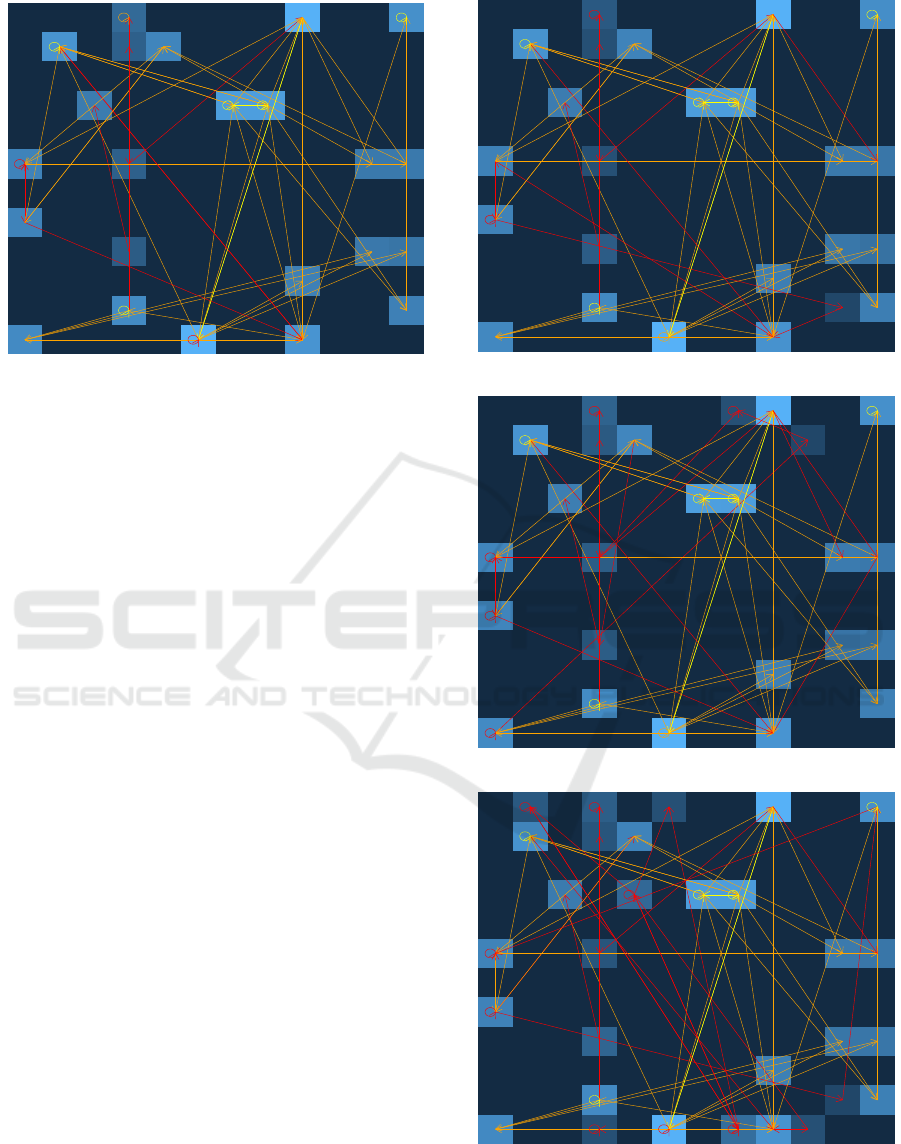
Figure 3: Visualization of syslog data representing normal
behavior.
which also includes the log data corresponding to the
attacks. Then, a sliding time window of 10 minutes
passes with a step width of 1 minute over all syslog
instances that occur before the first attack and maps
these points into the SOM. Figure 3 shows one of
these mappings. In the figure, some nodes are brighter
than others, meaning that they are hit more frequently.
Similarly, yellow arrows indicate a high number of
transitions between the two connected nodes, while
orange arrows indicate a moderate and red arrows a
low amount of transitions.
Despite the figure appearing complex at first
glance due to the many arrows overlapping, the to-
tal amount of arrows is comparatively low consider-
ing that transitions could exist between any of the 23
nodes active in this time window. In fact, the average
amount of outgoing transitions from each active node
is only 2.55. Comparing multiple visualizations of
non-overlapping time windows also shows that their
distributions of nodes and transitions is remarkably
consistent over time. This indicates that SOMs are
able to capture the normal system behavior correctly
and enables the detection of anomalies as changes of
the otherwise largely constant plot.
6.4 Anomaly Detection
As mentioned in the previous section, the log data
generated by the attacks was included in the training
input data. However, there does not exist a specific
feature that differentiates between normal and anoma-
lous input vectors as it is done in most supervised
learning methods that train their models on labeled
data. We therefore consider our proposed approach
to be an unsupervised method to identify anomalous
system behavior within a fixed set of input data that
a2_1000
sy_0
a0_d
a2_4000
sy_0
a0_d
mo_01006
sy_2
ou_0
a2_1000
a0_any
sy_0
og_33
ou_33
mo_01006
mo_01006
ou_33
sy_2
na_PAREN
it_2
mo_04173
a0_c
sy_0
a2_any
mo_01407
ou_105
og_112
mo_01407
ou_105
og_112
a2_1f40
a0_c
sy_0
a2_1f40
su_no
a0_c
sy_42
su_no
a0_any
sy_20
a0_c
a2_any
sy_20
a0_c
a2_any
su_no
a0_any
sy_0
mo_01207
sy_89
a2_1000
mo_01207
sy_89
a2_1000
na_UNKNO
su_no
sy_89
sy_49
a0_any
a2_any
a0_any
sy_1
a2_any
sy_42
a0_any
a2_any
sy_1
a2_any
a0_d
sy_0
a2_any
a0_d
Figure 4: Visualization of the local file inclusion attack.
a2_1000
sy_0
a0_d
a2_4000
sy_0
a0_d
mo_01006
sy_2
ou_0
a2_1000
a0_any
sy_0
mo_01006
ou_33
sy_2
na_PAREN
it_2
mo_04173
a0_c
sy_0
a2_any
mo_01407
ou_105
og_112
mo_01407
ou_105
og_112
a2_1f40
a0_c
sy_0
a2_1f40
su_no
a0_c
sy_42
su_no
a0_any
sy_20
a0_c
a2_any
sy_20
a0_c
a2_any
su_no
a0_any
sy_0
mo_01207
sy_89
a2_1000
mo_01207
sy_89
a2_1000
na_UNKNO
su_no
sy_89
sy_49
a0_any
a2_any
a0_any
sy_1
a2_any
sy_49
a2_any
a0_d
sy_42
a0_any
a2_any
sy_42
a2_any
a0_d
sy_1
a2_any
a0_d
sy_0
a2_any
a0_d
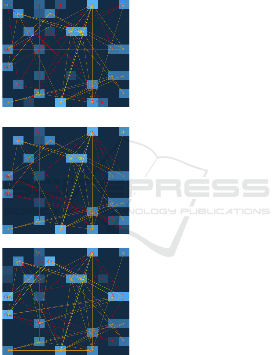
Figure 5: Visualization of the remote file inclusion attack.
a2_1000
sy_0
a0_d
pp_2004
co_id
ex_/usr/
a2_4000
sy_0
a0_d
pp_2004
co_id
ex_/usr/
mo_01006
sy_2
ou_0
ou_0
og_0
na_NORMA
a2_1000
a0_any
sy_0
og_33
ou_33
mo_01006
mo_01006
ou_33
sy_2
na_PAREN
it_2
mo_04173
a0_c
sy_0
a2_any
mo_01407
ou_105
og_112
mo_01407
ou_105
og_112
a2_1f40
a0_c
sy_0
a2_1f40
su_no
a0_c
sy_42
su_no
a0_any
sy_20
a0_c
a2_any
sy_20
a0_c
a2_any
su_no
a0_any
sy_0
pp_2004
co_id
ex_/usr/
mo_01207
sy_89
a2_1000
mo_01207
sy_89
a2_1000
na_UNKNO
su_no
sy_89
sy_49
a0_any
a2_any
a0_any
sy_1
a2_any
pp_2004
co_id
ex_/usr/
sy_42
a0_any
a2_any
a0_any
sy_1
a2_any
sy_1
a2_any
a0_d
sy_0
a2_any
a0_d
Figure 6: Visualization of the command injection attack.
enables clustering and differentiation between normal
behavior patterns and attack classes.
ICISSP 2020 - 6th International Conference on Information Systems Security and Privacy
356
a2_1000
sy_0
a0_d
sy_89
a2_1000
it_1
a2_4000
sy_0
a0_d
mo_01006
sy_2
ou_0
ou_0
og_0
na_NORMA
a2_1000
a0_any
sy_0
mo_01006
ou_33
sy_2
pp_2127
co_nc.tr
ex_/bin/
na_PAREN
it_2
mo_04173
a0_c
sy_0
a2_any
su_no
mo_01207
ou_0
mo_01407
ou_105
og_112
mo_01407
ou_105
og_112
a2_1f40
a0_c
sy_0
a2_1f40
su_no
a0_c
sy_42
su_no
a0_any
sy_20
a0_c
a2_any
sy_20
a0_c
a2_any
su_no
a0_any
sy_0
pp_2004
co_id
ex_/usr/
mo_01207
sy_89
a2_1000
mo_01207
sy_89
a2_1000
na_UNKNO
su_no
sy_89
sy_49
a0_any
a2_any
a0_any
sy_1
a2_any
pp_2127
co_nc.tr
ex_/bin/
sy_42
a0_any
a2_any
a0_any
sy_1
a2_any
sy_1
a2_any
a0_d
sy_0
a2_any
a0_d
Figure 7: Visualization of the remote command injection
attack.
a2_1000
sy_0
a0_d
a2_4000
sy_0
a0_d
mo_01006
sy_2
ou_0
sy_90
mo_01006
og_33
a2_1000
a0_any
sy_0
og_33
ou_33
mo_01006
mo_01006
ou_33
sy_2
na_PAREN
it_2
mo_04173
a0_c
sy_0
a2_any
mo_01407
ou_105
og_112
mo_01407
ou_105
og_112
a2_1f40
a0_c
sy_0
a2_1f40
su_no
a0_c
sy_42
su_no
a0_any
sy_20
a0_c
a2_any
sy_20
a0_c
a2_any
su_no
a0_any
sy_0
mo_01207
sy_89
a2_1000
mo_01207
sy_89
a2_1000
na_UNKNO
su_no
sy_89
sy_49
a0_any
a2_any
a0_any
sy_1
a2_any
sy_42
a0_any
a2_any
sy_1
a2_any
a0_d
sy_0
a2_any
a0_d
Figure 8: Visualization of the file upload injection scan.
a2_1000
sy_0
a0_d
a2_4000
sy_0
a0_d
mo_01006
sy_2
ou_0
a2_1000
a0_any
sy_0
og_33
ou_33
mo_01006
mo_01006
ou_33
sy_2
na_PAREN
it_2
mo_04173
a0_c
sy_0
a2_any
mo_01407
ou_105
og_112
mo_01407
ou_105
og_112
a2_1f40
a0_c
sy_0
a2_1f40
su_no
a0_c
sy_42
su_no
a0_any
sy_20
a0_c
a2_any
sy_20
a0_c
a2_any
na_UNKNO
su_no
na_any
su_no
a0_any
sy_0
su_no
sy_89
it_1
mo_01207
sy_89
a2_1000
mo_01207
sy_89
a2_1000
na_UNKNO
sy_20
a0_c
na_UNKNO
sy_2
su_no
na_UNKNO
su_no
sy_89
sy_49
a0_any
a2_any
a0_any
sy_1
a2_any
sy_42
a0_any
a2_any
sy_1
a2_any
a0_d
sy_0
a2_any
a0_d
Figure 9: Visualization of the vulnerability scan.
We now go through the SOM visualizations that
involve attacks. For this, the sliding window approach
used to capture the normal system behavior was car-
ried on to generate SOM mappings for time windows
of 10 minutes length distributed over the whole data
set. We compared the consecutive SOM visualiza-
tions to empirically assess that this time window size
is large enough to record almost all normal behavior
and small enough so that attacks do not overlap, i.e.,
there is always at most one attack taking place in ev-
ery time window. Also note that the maximum delay
between the launch of the attacks and their detection
is equal to the step width of the sliding time window,
i.e., in our setting, it takes at most 1 minute after com-
pletion of the attack to see its effects in the SOM. In
the following, we select a representative time window
for each attack and discuss whether and how the ma-
licious behavior manifests itself as artifacts in the re-
spective visualizations.
Figure 4 shows the visualization of the system be-
havior influenced by the local file inclusion attack.
This attack only generates a single suspicious syscall
log line and is thus the most difficult attack to detect
for our SOM approach. Comparing the SOM map-
pings to the SOM that visualizes normal behavior,
this log line manifests itself as one additional node hit
that is visible close to the bottom right corner of the
SOM. The labels suggest that ogid=33, ouid=33, and
mode=0100644 are the most relevant features. We
assessed that these feature values individually occur
several thousand times in the data, but only their com-
bined occurrence is distinctive for this and three other
attacks. This shows that the attack is not detectable
by monitoring all parameter values individually, but
only the combinations of values.
As visible close to the top right corner of the SOM
in Fig. 5, the remote file inclusion attack includes
the execution of syscall types 42 and 49. Again, both
these syscalls and the parameter a0=d are common
in the data, but only their combined occurrences are
unique for this attack. The command injection at-
tack displayed in Fig. 6 is easier to detect, since it
generates several unusually parameterized log lines,
which are visible in the top and bottom of the SOM.
In particular, the log lines stand out due to their parent
process id (ppid) of 2004 and the command (comm)
value “id”. A similar interpretation is possible for the
remote command injection attack displayed in Fig. 7,
with the difference that netcat (nc.traditional) is used
as a command. Figure 8 shows the file upload injec-
tion attack, which causes the execution of the same
command as the local file inclusion attack and addi-
tionally generates a syscall of type 90 that appears
as a node hit in the bottom right of the SOM. This
Visualizing Syscalls using Self-organizing Maps for System Intrusion Detection
357
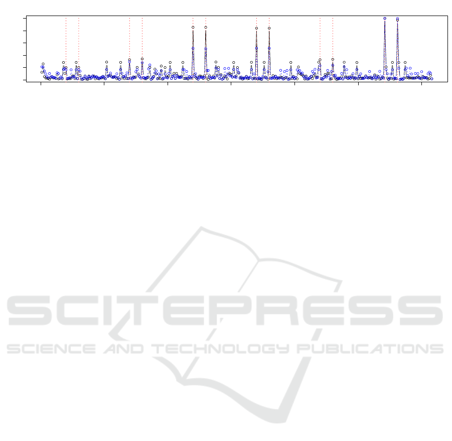
0 50 100 150 200 250 300
0.0 0.2 0.4 0.6 0.8 1.0
Node and Transition Changes between Time Windows
Time window
Anomaly Score
Figure 10: Anomaly scores computed from node (solid black line) and transition (dashed blue line) changes show rapid
increases when the sliding time window enters and leaves intervals containing attacks (dotted red, vertical lines).
is the only syscall of this type in the data and thus
also detectable without context information. Finally,
Fig. 9 shows the SOM corresponding to the vulnera-
bility scan. This attack induces the execution of sev-
eral thousand syscalls and is thus the easiest of our
attacks to detect. Beside some previously inactive
nodes receiving hits, the attack mainly manifests it-
self as changes of hit and transition frequencies in the
SOM, visible by nodes turning brighter and arrows
changing color.
As outlined in Sect. 5.3, the differences between
the consecutively generated SOMs result in time-
series that indicate changes of system behavior. Fig-
ure 10 shows the progression of these anomaly scores
measured on the nodes and transitions over time. Note
that due to our sliding window approach, each at-
tack causes a peak when the attack enters the window
and another one when the attack leaves the window.
The anomaly score does not indicate system behav-
ior changes from time windows in-between, because
they are all equally affected by the same attack. The
dashed red lines mark the points in time where the
change of system behavior is expected.
In alignment with the observed changes of the
SOMs, the third, fourth and sixth attack are strongly
visible as peaks of the anomaly score, the second
and fifth attack cause moderate increases and the first
attack slight increases of the anomaly score. The
progression of the anomaly score also shows several
smaller peaks that are dismissed as false positives.
Closer inspection shows that most of them are indeed
generated by inconsistent behavior of the web server,
but do not relate to our injected attacks.
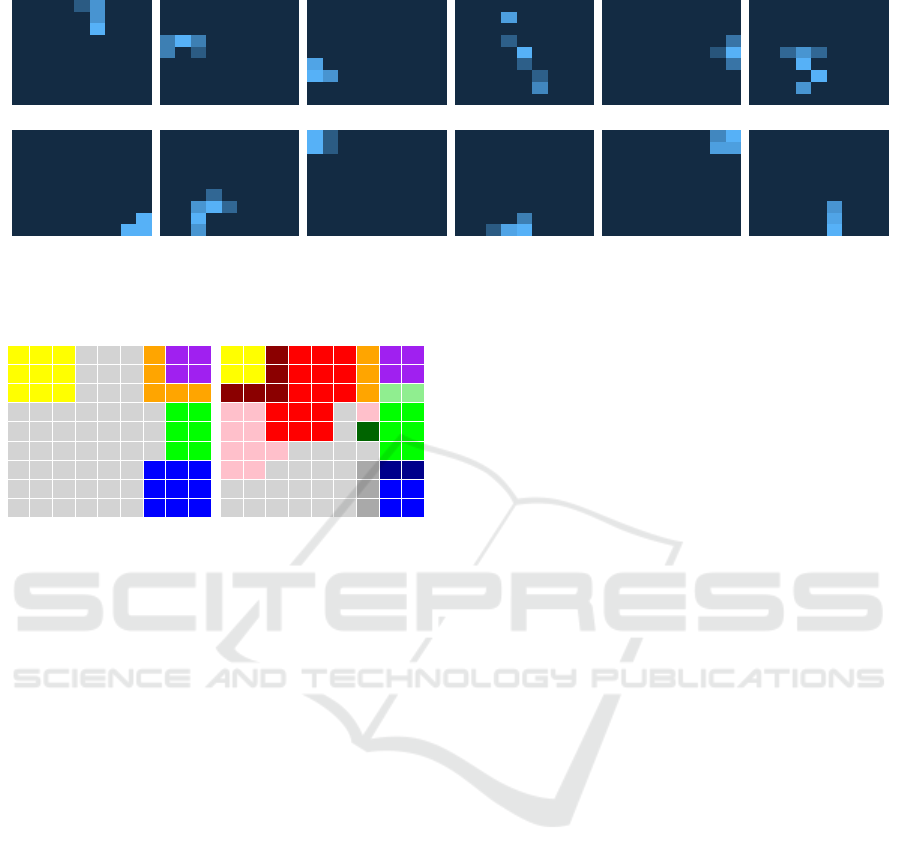
Finally, Fig. 11 shows the results of our exper-
iments with aggregated syscall data as described in
Sect. 5.4. We display twelve plots where attack and
normal behavior phases are alternating, i.e., the plots
in the first, third, and fifth column correspond to the
six attacks, while the plots in the second, fourth, and
sixth column correspond to phases of normal behavior
in between. Note that each plot covers a time span of
35 minutes and consists of data points that represent
25 minute time windows, e.g., the first plot covers the
time span of minute 7 to 42 and contains twelve data
points corresponding to the sliding time windows 7-
32 minutes, 8-33 minutes, ..., 18-43 minutes.
We interpret the plots as follows. Time windows
of normal system behavior relate to nodes in the cen-
ter or closer to the bottom left of the plot. Time win-
dows that contain attacks end up concentrated on the
sides or in the corners of the SOM. The reason for
this is that these anomalous phases are highly differ-
ent and thus end up far away from the normal behav-
ior. The reason that the normal behavior does not per-
fectly overlap is attributable to the false positives al-
ready mentioned.
Note that we ascertained that the labels largely
correspond to the labeling of the SOMs discussed be-
fore, i.e., nodes of SOM mappings of data containing
attacks are labeled according to the respective features
relevant for detection. For a more convenient view of
the plots, we decided to cluster the nodes according
to their distances using a hierarchical clustering al-
gorithm. The clusters are displayed in Fig. 12 for a
predefined amount of 6 clusters (left) and 13 clusters
(right). Note that the cluster plot functions as a mask
that classifies system behavior when being superim-
posed on the SOMs from Fig. 11. In particular, the
left plot shows that clusters are found at the top left,
top right, and bottom right corner as well as the right
edge of the SOM, while the large gray area (marked
with 1) mostly corresponds to normal behavior. The
colored areas correspond to the third, fourth, fifth, and
sixth attack, and thus confirm our interpretations of
the SOMs. Note that the clusters 5 and 6 in the top
right corner correspond to only one attack. The plot
on the right shows that a more fine-grained cluster-
ing is required to also identify the first and second
attack, which are more difficult to detect. However,
this also misclassifies the normal behavior between
the first and second attack.
ICISSP 2020 - 6th International Conference on Information Systems Security and Privacy
358
Time window 7 − 42
Time window 36 − 71
Time window 61 − 96
Time window 89 − 124
Time window 113 − 148
Time window 139 − 174
Time window 169 − 204
Time window 193 − 228
Time window 214 − 249
Time window 237 − 272
Time window 267 − 302
Time window 283 − 318
Figure 11: SOMs of aggregated syscall data from multiple time spans. The plots in the first, third, and fifth columns cor-
respond to attack time windows, while the plots in the second, fourth, and sixth columns correspond to normal behavior in
between.
1 1 1 1 1 1 2 2 2
1 1 1 1 1 1 2 2 2
1 1 1 1 1 1 2 2 2
1 1 1 1 1 1 1 3 3
1 1 1 1 1 1 1 3 3
1 1 1 1 1 1 1 3 3
4 4 4 1 1 1 5 5 5
4 4 4 1 1 1 5 6 6
4 4 4 1 1 1 5 6 6
1 1 1 1 1 1 10 2 2
1 1 1 1 1 1 10 2 2
12 12 1 1 1 1 10 13 13
12 12 12 1 1 1 1 3 3
12 12 7 7 7 1 8 3 3
12 12 7 7 7 1 12 3 3
9 9 9 7 7 7 5 11 11
4 4 9 7 7 7 5 6 6
4 4 9 7 7 7 5 6 6
Figure 12: Clusters serving as a mask for SOMs. Left: 6
clusters differentiate normal behavior (marked with 1) and
four attack phases. Right: 13 clusters identify all attack
phases.
7 DISCUSSION
The results presented in the previous section show
that all injected attacks are detected by our approach.
In particular, the labels of the nodes that correspond
to the anomalies indicate that the parameters of the
syscall log lines are essential in differentiating be-
tween normal and anomalous behavior. This is a sig-
nificant advantage to existing methods that only focus
on syscall types alone.
Employing SOMs for system behavior modeling
emerged as a useful tool to generate visual assis-
tance that improves the overview of the data and en-
ables the exploratory detection of anomalous behav-
ior. Thereby, no particular domain knowledge about
the syscall log lines and the monitored system itself
is required, as long as a reasonable time window size
that captures all normal behavior is selected. We de-
liberately did not select a particular set of parame-
ters for our analyses, but rather used all available val-
ues that occur sufficiently many times in the data,
as outlined in Sect. 3.2. We realize that difficulties
regarding the selection of appropriate time window
sizes and thresholds for binning feature values may
emerge in practical applications, but argue that they
can be determined with reasonable effort during the
exploratory analysis. Nevertheless, we are aware that
an automated parameter selection is able to improve
the method and support the analyst. We leave this task
for future work.
Despite the fact that our feature selection com-
bined with the one-hot encoding resulted in high-
dimensional input vectors, we observed that the com-
plexity of the data was rather low, consisting only of
70 unique types of input vectors. The reason for this
is that our Apache server handles almost all opera-
tions made on the website similarly, despite random
navigation and selections on the website. A system
that produces more complex input data would require
larger SOM sizes in order to decrease the chance of
normal and attack input vectors being mapped to the
same nodes. Choosing optimal SOM sizes and cutoff
values for feature selection is non-trivial and must be
determined iteratively by exploration. Note that we
due to our exploratory approach, we did not carry out
any evaluation regarding the computation time and fo-
cused on the detection and interpretation of patterns.
One limitation of our approach is that attack vec-
tors must be present in the training data, otherwise the
SOM does not learn the feature weights of the attacks,
and mapping them to specific nodes is not possible.
This prevents online detection of unknown anomalies
on a pre-trained SOM. One solution is to continuously
retrain a SOM on the most recent data for detection of
unknown anomalies and use pre-trained SOMs only
for classification of known attacks.
Furthermore, it is non-trivial to derive concise
rules that describe system behavior from SOMs. This
is due to the fact that the visualized processes fre-
quently overlap partially and share nodes, making it
difficult to extract dependencies.
Finally, the node placement of SOMs is topolog-
ically correct in the sense that similar syscalls are
likely to be located close to each other. This makes
Visualizing Syscalls using Self-organizing Maps for System Intrusion Detection
359

it possible to easily recognize variations of existing
sequences and determine which features are respon-
sible for the divergences. However, the placement
is almost certainly not ideal to visualize syscall se-
quences in chains, i.e., to reduce the arrow lengths
between nodes. While it is possible to display the ac-
tive nodes of a SOM and their transitions as a graph
and reorder the nodes to avoid edges crossing over
or running across the plot, this would undermine the
topological node placement of the SOM.
We especially recommend our approach for sys-
tems with predictable behavior, otherwise the amount
of false positives may easily become overwhelming.
8 CONCLUSION
In this paper, we introduced an approach to visu-
alize high-dimensional syscall log lines using self-
organizing maps. Other than most existing ap-
proaches, our solution incorporates parameters as
context information, which is necessary to identify at-
tacks that do not manifest themselves as anomalous
sequences of syscall types, but rather involve unusual
combinations of parameter values. Our visualizations
involve hit histograms that show the number of input
vectors mapped to each node, as well as transitions
that display hit sequences. We used a sliding window
approach to analyze consecutively generated SOMs
and computed an anomaly score based on their pair-
wise changes. In addition, we proposed to aggregate
the syscalls within time windows and also visualized
their occurrence counts. We generated syscalls on a
real system to validate our approach. All attacks in-
jected in the system were identified as changes of the
SOMs. We therefore conclude that SOMs are suitable
to be applied for semi-automatic anomaly detection
in fixed data sets by supporting exploratory analyses
with visual cues.
ACKNOWLEDGEMENTS
This work was partly funded by the FFG projects IN-
DICAETING (868306) and DECEPT (873980), and
the EU H2020 project GUARD (833456).
REFERENCES
Abed, A. S., Clancy, T. C., and Levy, D. S. (2015). Ap-
plying bag of system calls for anomalous behavior de-
tection of applications in linux containers. In IEEE
Globecom Workshops, pages 1–5. IEEE.
Chandola, V., Banerjee, A., and Kumar, V. (2009).
Anomaly detection: A survey. ACM Computing Sur-
veys, 41(3):15.
Creech, G. and Hu, J. (2014). A semantic approach to host-
based intrusion detection systems using contiguous
and discontiguous system call patterns. IEEE Trans-
actions on Computers, 63(4):807–819.
Eskin, E., Lee, W., and Stolfo, S. (2001). Modeling sys-
tem call for intrusion detection using dynamic window
sizes. Proceedings DARPA Information Survivability
Conference and Exposition II, pages 165–175.
Forrest, S., Hofmeyr, S. A., Somayaji, A., and Longstaff,
T. A. (1996). A sense of self for unix processes. In
Proceedings of the IEEE Symposium on Security and
Privacy, pages 120–128. IEEE.
Girardin, L. and Brodbeck, D. (1998). A visual approach for
monitoring logs. In Proceedings of the 12th Systems
Administration Conference, pages 299–308.
Harris, D. M. and Harris, S. L. (2007). Chapter 3 - se-
quential logic design. In Digital Design and Com-
puter Architecture, pages 103 – 165. Morgan Kauf-
mann, Burlington.
Kavanagh, K., Bussa, T., and Sadowski, G. (2018). Magic
quadrant for security information and eventmanage-
ment. Gartner.
Kim, G., Yi, H., Lee, J., Paek, Y., and Yoon, S. (2016).
Lstm-based system-call language modeling and robust
ensemble method for designing host-based intrusion
detection systems. arXiv preprint.
Kohonen, T. (1982). Self-organized formation of topolog-
ically correct feature maps. Biological Cybernetics,
43:59–69.
Liu, A., Jiang, X., Jin, J., Mao, F., and Chen, J. (2011). En-
hancing system-called-based intrusion detection with
protocol context. pages 103–108.
Mandal, S. (2018). Operating system — introduc-
tion of system call. https://www.geeksforgeeks.org/
operating-system-introduction-system-call/. Online;
accessed: 2019-12-04.
Saxe, J., Mentis, D., and Greamo, C. (2012). Visualization
of shared system call sequence relationships in large
malware corpora. In Proceedings of the 9th Interna-
tional Symposium on Visualization for Cyber Security,
pages 33–40. ACM.
Shu, X., Yao, D., and Ramakrishnan, N. (2015). Un-
earthing stealthy program attacks buried in extremely
long execution paths. In Proceedings of the 22nd ACM
SIGSAC Conference on Computer and Communica-
tions Security, pages 401–413. ACM.
Skopik, F., Settanni, G., Fiedler, R., and Friedberg, I.
(2014). Semi-synthetic data set generation for secu-
rity software evaluation. In Proceedings of the 12th
Annual International Conference on Privacy, Security
and Trust, pages 156–163. IEEE.
Yoon, M.-K., Mohan, S., Choi, J., Christodorescu, M., and
Sha, L. (2017). Learning execution contexts from sys-
tem call distribution for anomaly detection in smart
embedded system. In Proceedings of the 2nd Interna-
tional Conference on Internet-of-Things Design and
Implementation, pages 191–196. ACM.
ICISSP 2020 - 6th International Conference on Information Systems Security and Privacy
360
