
Improved Subspace Method for Supervised Anomaly Detection with
Minimal Anomalous Data
Fumito Ebuchi
a
, Aiga Suzuki
b
and Masahiro Murakawa
c
Graduate School of Systems and Information Engineering, University of Tsukuba, Japan
National Institute of Advanced Industrial Science and Technology (AIST), Japan
Keywords:
Subspace Method, Anomaly Detection, Optimization Problems.
Abstract:
In conventional anomaly detection methods, the classifier is usually trained only with normal data. How-
ever, real-world problems may present a very small amount of anomalous data. In this paper, we propose
an improved subspace method for anomaly detection that has the ability to utilize a very small amount of
anomalous data. Our method introduces an objective function that minimizes the average projection length
of anomalous data into the conventional objective function for the subspace method. This formulation en-
ables a normal subspace that considers the distribution of anomalous data to be learned, thereby improving
the anomaly detection performance. Furthermore, because the information about anomalous data is provided
in the form of the average projection length, stable detection can be expected even when an extremely small
amount of anomalous data is used. We used MNIST and the CIFAR-10 dataset to evaluate the effectiveness
of the proposed method, which yielded a higher anomaly detection performance compared with the conven-
tional normal model or classifier model under conditions in which very little anomalous data are obtainable.
The performance of our method on CIFAR-10 was assessed by imposing the constraint that only four or five
anomalous data samples could be used. In this test, our method achieved an average AUC of 0.263 points
higher than that of the state-of-the-art method using only normal data.
1 INTRODUCTION
The subspace method (SM)(Watanabe and Pakvasa,
1973; Oja, 1983), which is a pattern recognition tech-
nique, generates a low-dimensional subspace that rep-
resents the data distribution. In other words, the
subspace contains the maximum projection length of
data. Therefore, the optimization of SM entails the
maximization of the average projection length of data
onto its surface. In classification problems, the in-
put data are classified into the class with the highest
similarity between the input data and the class sub-
space, which can be obtained from the data of one
class. Therefore, SM can also be applied to one-class
classification problems and anomaly detection prob-
lems.
On the other hand, the decreasing cost of col-
lecting sensor data has prompted active research
on anomaly detection using machine-learning tech-
a
https://orcid.org/0000-0002-7982-0436
b
https://orcid.org/0000-0002-7794-1162
c
https://orcid.org/0000-0002-8406-7426
niques. This approach to anomaly detection has been
used for machine failure detection(Hasegawa et al.,
2018), fault detection in parts manufacturing(Moyne
and Iskandar, 2017), the detection of attacks in net-
work security(Barford et al., 2002), and the detec-
tion of anomalous echoes in infrastructure equipment
inspection(Ye et al., 2014). In general, in the field
of anomaly detection, anomalous data are difficult
to obtain compared to normal data, of which a large
amount is available. Therefore, most anomaly detec-
tion techniques using machine learning train a nor-
mal state using only normal data, and detect anoma-
lous data based on the dissimilarity from the normal
state(Wang et al., 2004)(An and Cho, 2015)(Zhou and
Paffenroth, 2017). Semi-Supervised Anomaly De-
tection (SSAD)(G
¨
ornitz et al., 2013) is a valuable
anomaly detection method that can utilize anomaly
data based on Support Vector Data Description (Tax
and Duin, 2004). SSAD generates hyperspheres that
contain normal data and no anomalous data. SSAD
is effective when we have a large amount of anoma-
lous data, but is ineffective when very little anoma-
lous data are available. However, real-world problems
Ebuchi, F., Suzuki, A. and Murakawa, M.
Improved Subspace Method for Supervised Anomaly Detection with Minimal Anomalous Data.
DOI: 10.5220/0008918401510158
In Proceedings of the 9th International Conference on Pattern Recognition Applications and Methods (ICPRAM 2020), pages 151-158
ISBN: 978-989-758-397-1; ISSN: 2184-4313
Copyright
c
2022 by SCITEPRESS – Science and Technology Publications, Lda. All rights reserved
151

involve very small amounts of anomalous data in ad-
dition to a large amount of normal data. Therefore,
if we were to succeed in using these anomalous data
effectively, the anomaly detection performance could
be improved compared to the conventional anomaly
detection method.
In this paper, we propose a supervised SM with
a large amount of normal data and very little anoma-
lous data. The objective function of the conventional
SM is to maximize the average projection length of
normal data. The proposed method contains an addi-
tional term, which is added to minimize the average
projection length of very little anomalous data to the
objective function of the conventional SM. The eigen-
value problem is derived by applying the Lagrange
multiplier method to the optimization problem. Then,
we can obtain a basis vector of the normal class sub-
space by solving the eigenvalue problem. The pro-
posed method detects the anomalous data based on
the projection length when an unknown data value is
projected into the normal class subspace. Because
the normal class subspace of the proposed method
considers the distribution of anomalous data, it can
be expected to improve the anomaly detection per-
formance. Furthermore, even when extremely little
anomalous data are available, we expect to be able to
utilize these anomalous data to stably detect anoma-
lous data. This expectation considers that the pro-
posed method provides information on the anomalous
data using the average projection length.
In this paper, in Sect. 2, we discuss the necessi-
ties of anomaly detection with a large amount nor-
mal data and a small amount of anomalous data, and
describe the conventional SM. In Sect. 3, we present
the proposed method, and in Sect. 4, we describe the
effectiveness of the proposed method, which was as-
sessed by conducting computer experiments using the
MNIST and CIFAR-10 datasets. In Sect. 5, we deliver
the conclusion.
2 BACKGROUND AND RELATED
WORK
Anomaly detection has been studied for a long time,
and many anomaly detection methods have been pro-
posed. However, because anomalous data rarely ap-
pear in real-world problems, most anomaly detec-
tion methods are trained only with normal data. In
fact, it is rarely possible to obtain more than small
amounts of anomalous data. We could therefore ex-
pect to improve the anomaly detection performance
by utilizing the rare anomalous data instead of nor-
mal data. In such cases, we could use binary clas-
sifiers such as neural networks, a support vector ma-
chine, and random forest without using an anomaly
detection method. However, a binary classifier can-
not detect unknown data that are not contained in the
training dataset. Furthermore, it would not be pos-
sible to train the classifier thoroughly because of the
data bias. Therefore, we would need to devise a way
to use the small amount of anomalous data effectively,
to enable the anomaly detection method to generate a
normal state.
Typical anomaly detection methods include a one-
class support vector machine, auto-encoder, and SM.
Among these methods, SM has been widely used be-
cause of its high generalization ability and easy im-
plementation. In this section, we describe the con-
ventional SM for anomaly detection in detail.
2.1 Subspace Method
In anomaly detection, we obtain the subspace for the
normal data by solving the following optimization
problem.
maximize
1
|S
+
|
∑
i∈S
+
(x
>
i
v)
2
(1)
subject to v
>
v = 1, (2)
where x, v, and S
+
are the l-dimensional input vector,
l-dimensional weight vector, and subscript indicates
the subset of normal data, respectively. Introducing a
Lagrange multiplier λ enables equation (1) and (2) to
be transformed into the following optimization prob-
lem:
maximize
1
|S
+
|
∑
i∈S
+
(x
>
i
v)
2
− λ(v
>
v − 1). (3)
The optimal condition for v can be obtained by the
following eigenvalue problem,
1
|S
+
|
∑
i∈S
+
x
i
x
>
i
v = λv. (4)
We can obtain l eigenvalues λ
1
, λ
2
, ··· , λ
l
(λ
1
≥
λ
2
≥ · · · ≥ λ
l
) and corresponding l eigenvectors
v
1
, v
2
, ··· , v
l
by solving the eigenvalue problem of
equation (4). Because these eigenvectors contain re-
dundant expressions, we select eigenvectors that sat-
isfy the following equation.
∑
r
i=1
λ
i
∑
l
i=1
λ
i
≥ η, (5)
where η is a hyperparameter less than 1, a so-called
cumulative contribution rate. Then, we find the
smallest r that satisfies equation (5), and define V =
ICPRAM 2020 - 9th International Conference on Pattern Recognition Applications and Methods
152

(v
1
, v
2
, ··· , v
r
), where r < l as the normal class sub-
space.
The anomaly score of data z is calculated as the
distance between z and ˆz, which is reconstructed by
subspace V . In other words, the anomaly score is:
D
+
(z) = |sin θ|
=
kz − ˆzk
2
kzk
2
=
k(I
l×l
−VV
>
)zk
2
kzk
2
, (6)
where I
l×l
is an l × l identity matrix. Data z with a
relatively large D
+
(z) in equation (6) is classified as
anomalous data.
3 PROPOSED METHOD
In the conventional SM, the normal subspace is gen-
erated using normal data only. Therefore, even if we
were able to obtain anomalous data, we would not
be able to utilize these data. Thus, the effective use
of anomalous data would be expected to improve the
anomaly detection performance. Therefore, we de-
fine a formulation by considering the anomalous data.
Specifically, we introduce a condition that minimizes
the average projection length of the anomalous data
to the objective function of the conventional equation
(1) as follows:
maximize
1
|S
+
|
∑
i∈S
+
(x
>
i
v)
2
−
C
|S
−
|
∑
i∈S
−
(x
>
i
v) (7)
subject to v
>
v = 1, (8)
where C ∈ R
+
, and S
−
are the tradeoff hyperparame-
ters between the normal and anomalous data, and the
subscript subset of the anomalous data, respectively.
Especially, in the case of C = 0, equation (7) is equal
to equation (1). As in Sect. 2, we can obtain the
following eigenvalue problem by introducing the La-
grange multiplier λ into equation (7) and (8).
1
|S
+
|
∑
i∈S+
x
i
x
>
i
−
C
|S
−
|
∑
i∈S
−
x
i
x
>
i
v = λv (9)
By solving equation (9), we obtain eigenvectors
v
1
, v
2
, ··· , v
l
. Therefore, as in the conventional SM,
we obtain subspace V = (v
1
, v
2
, ··· , v
r
) using equa-
tion (5). In equation (7), because we use the infor-
mation on anomalous data by employing the average
projection length, it becomes possible to utilize very
little anomalous data in an effective manner.
The illustration in Figure 1 compares the conven-
tional subspace with the subspace of the proposed
method. Because the conventional subspace is deter-
mined only by normal data, anomalous data cannot be
considered. However, the proposed method considers
anomalous data, and designates an area away from the
data known to be anomalous as the normal subspace.
The generation of such a normal subspace enables the
anomaly detection performance to be improved.
T
5
T
Ü
T
ß?5
T
ß
Conventional SM
Known anomalous data
Proposed method
€
€
€
€
Known normal data
move
Figure 1: Comparison of the proposed method and conven-
tional SM.
4 EXPERIMENTS AND RESULTS
We demonstrate the effectiveness of the proposed
method using the MNIST and CIFAR-10 datasets.
Because the proposed method uses very little anoma-
lous data, we compared the performance on both
of these datasets using both an anomaly detection
method and a binary classifier.
4.1 Methods
We compare the proposed method with the conven-
tional SM with only normal data, and convolutional
neural network ResNet-50(He et al., 2016) as a binary
classifier. In this section, we refer to the proposed
method as “ISM”, and ResNet-50 for a binary clas-
sifier as “BI-ResNet-50”. For SM and ISM, we used
the features of the fully connected layer of ResNet-
50 as the input features. In this section, we refer to
the feature extractor using ResNet-50 as “FE-ResNet-
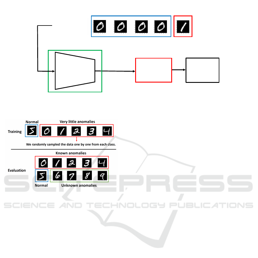
50”. Figure 2 shows the flow of the proposed method.
In addition, we compare the proposed method and
SSAD(G
¨
ornitz et al., 2013), which is trained with
both normal and anomalous data.
Furthermore, we compared the results of the
aforementioned methods with those of ISM, to
demonstrate the performance of our method relative
to the following recently proposed well-known meth-
ods that use only normal data.
Improved Subspace Method for Supervised Anomaly Detection with Minimal Anomalous Data
153
Pre-trained
CNN model
(ResNet50)
>rás?
Feature Extractor
Normalization
Proposed
Method
(ISM)
Anomaly
Score
&
>
:V;
Training data :
A large amount of normal data
Very little
anomalous data
Figure 2: Flow of the proposed method.
Figure 3: Experimental setting for training and test data
with anomalous data.
• Kernel Density Estimation (KDE) (Parzen,
1962)
• One-Class Support Vector Machine (OC-
SVM) (Scholkopf and Smola, 2001)
• Isolation Forest (IF) (Liu et al., 2008)
• Gaussian Mixture Model (GMM) (Fraley and
Raftery, 2002)
• Deep Convolutional Autoencoder (DCAE)
(Masci et al., 2011)
• Anomaly Detection with Generative Adversar-
ial Network (AnoGAN) (Schlegl et al., 2017)
• Variational Autoencoder (VAE) (Kingma and
Welling, 2013)
• Anomaly Detection with Generative Adversar-
ial Network (ADGAN) (Deecke et al., 2018)
The experimental results of each of these methods
were surveyed from (Deecke et al., 2018).
4.2 Setting Hyperparameters
We fine-tuned all the layers of BI-ResNet-50 for 20
epochs using an Adam optimizer (α = 0.001, β
1
=0.9,
β
2
=0.999, ε = 10
−8
) and the weighted cross entropy
loss for considering class imbalance. The initial value
of BI-ResNet-50 is the weight and bias pre-trained
with ImageNET(Deng et al., 2009). FE-ResNet50
had pre-trained weights with ImageNET, and did not
require fine-tuning.
The hyperparameters used in SSAD, SM, and
ISM were selected by 4-FOLD cross validation.
In our experiment, because there are only 4 or 5
anomalous data in the training data, we divided
the training data 3:1 for normal data and 1:3 for
anomalous data, and cross-validated with AUC as
the evaluation value. The hyperparameters were
selected every time the training dataset changed. We
selected η from {0.80, 0.85, 0.90, 0.95, 0.99}, C from
{0.5, 0.4, 0.3, 0.2, 0.1, 0.09, 0.08, 0.07, 0.06, 0.05, 0.04,
0.03, 0.02, 0.01}, the RBF kernel parameter
γ from {0.01, 0.1, 1, 10, 100}, and the trade-
off parameter for the error in SSAD from
{10
−2
, 10
−1
, 10
0
, 10
1
, 10
2
, 10
3
}. We set the trade-off
parameter for the margin κ = 1.0.
4.3 Datasets
We assessed the performance using the above-
mentioned two popular datasets. The first, the MNIST
dataset, which contains grayscale images of handwrit-
ten digits, contains 60,000 training images and 10,000
test images with a 28 × 28 image size. The other,
the CIFAR-10 dataset, which contains RGB images
of real-world objects belonging to ten classes, con-
tains 50,000 training images and 10,000 test images
with an image size of 32 × 32.
ICPRAM 2020 - 9th International Conference on Pattern Recognition Applications and Methods
154

Table 1: Comparison of average AUC.
Normal Binary classification Semi-Supervised Ours
Dataset class ResNet50 SM SSAD ISM
0 0.979±0.015 0.944±0.037 0.981±0.017 0.988±0.003
1 0.973±0.026 0.993±0.004 0.999±0.000 0.999±0.000
2 0.948±0.031 0.814±0.067 0.911±0.025 0.932±0.020
3 0.960±0.025 0.857±0.054 0.935±0.000 0.946±0.014
MNIST 4 0.983±0.007 0.928±0.038 0.960±0.019 0.983±0.006
5 0.953±0.021 0.831±0.048 0.926±0.000 0.937±0.015
6 0.994±0.003 0.837±0.064 0.932±0.000 0.956±0.011
7 0.967±0.024 0.874±0.069 0.940±0.023 0.975±0.006
8 0.969±0.023 0.903±0.062 0.974±0.000 0.977±0.006
9 0.924±0.037 0.858±0.055 0.890±0.034 0.958±0.008
Avg. 0.965±0.019 0.884±0.054 0.945±0.032 0.965±0.021
Airplane 0.700±0.074 0.790±0.088 0.880±0.034 0.895±0.005
Automobile 0.859±0.035 0.893±0.021 0.927±0.017 0.938±0.005
Bird 0.635±0.057 0.724±0.034 0.826±0.041 0.820±0.019
Cat 0.642±0.057 0.732±0.061 0.812±0.017 0.831±0.023
CIFAR-10 Deer 0.699±0.050 0.754±0.081 0.803±0.038 0.845±0.024
Dog 0.741±0.040 0.847±0.026 0.903±0.000 0.905±0.009
Frog 0.781±0.039 0.858±0.052 0.923±0.034 0.942±0.008
Horse 0.782±0.023 0.855±0.056 0.913±0.031 0.923±0.005
Ship 0.748±0.058 0.856±0.082 0.911±0.018 0.925±0.010
Truck 0.823±0.028 0.854±0.098 0.930±0.025 0.945±0.011
Avg. 0.741±0.069 0.816±0.058 0.883±0.047 0.897±0.045
4.4 Experimental Setting
Suppose we have a large amount of normal data and
very little anomalous data in the training dataset. In
our experiment, we assumed the data in each single
class to be normal. The training dataset contained a
large number of images from this single class. Addi-
tionally, we randomly sampled data one by one from
other class numbers as anomalous data. That is, the
number of anomalous data is very small compared to
the number of normal data in the training dataset.
Figure 3 shows the experimental setting for the
training and test data with anomalies for the MNIST
dataset. In this example, we take class5 as a normal
class, and one image of each of classes 0, 1, 2, 3, and
4 as anomalous data for the training dataset. The eval-
uation covered the data in all classes. In other words,
class 5, class 0, 1, 2, 3, and 4, and class 6, 7, 8, and 9
are a normal class, known anomaly classes, unknown
anomaly classes, respectively.
In the experiments, we define half of all classes
as known anomalies which are included in the train-
ing dataset. For the MNIST data set, we set known
anomalies as class 0, 1, 2, 3, and 4. For the CIFAR-
10 dataset, we set known anomalies as the airplane,
automobile, bird, cat, and deer classes. In the case
the normal class is included in the known anomalies
classes , the normal class is excepted from the anoma-
lies. Therefore, the training dataset included four or
five anomalous data and a large number of normal
data.
The random selection of anomalous data was
achieved by repeatedly evaluating the classifier that
uses the anomalous data for training ten times under
the same experimental conditions, and comparing it
with the average value. The experiment was evalu-
ated using AUC for all test data.
4.5 Experimental Results
Table 1 lists the AUC for each problem for the con-
ventional and the proposed methods. The maximum
AUC for each problem is shown in bold. “Avg.”
means the average AUC for all classes. The experi-
ments were repeated ten times for the method using
the anomalous data, and the standard deviation is pro-
vided in the table.
For the MNIST dataset, the AUC for ISM is im-
proved by 0.081 points on average, compared with
the conventional SM. Because ISM minimizes the av-
erage projection length of anomalous data, a normal
subspace is generated away from the anomalous data.
A comparison of the AUC for ISM and ResNet-50
reveals that the average AUC for for the two meth-
ods is the same. Because the classification of the data
in MNIST is a simple problem, it is possible to de-
Improved Subspace Method for Supervised Anomaly Detection with Minimal Anomalous Data
155

Table 2: Comparison of average AUC for known and unknown anomalies.
Normal All data vs. Known anomalies vs. Unknown anomalies
Dataset class SM ISM ISM ISM
0 0.944±0.037 0.988±0.003 0.995±0.002 0.98±0.004
1 0.993±0.004 0.999±0.000 0.999±0.000 0.999±0.001
2 0.814±0.067 0.932±0.020 0.940±0.017 0.935±0.023
3 0.857±0.054 0.946±0.014 0.962±0.013 0.958±0.012
MNIST 4 0.928±0.038 0.983±0.006 0.985±0.009 0.98±0.004
5 0.831±0.048 0.937±0.015 0.920±0.018 0.960±0.011
6 0.837±0.064 0.956±0.011 0.951±0.012 0.963±0.009
7 0.874±0.069 0.975±0.006 0.966±0.010 0.987±0.002
8 0.903±0.062 0.977±0.006 0.978±0.005 0.975±0.008
9 0.858±0.055 0.958±0.008 0.968±0.007 0.944±0.010
Avg. 0.884±0.054 0.965±0.021 0.966±0.023 0.968±0.019
Airplane 0.790±0.088 0.895±0.005 0.916±0.005 0.859±0.007
Automobile 0.893±0.021 0.938±0.005 0.976±0.005 0.888±0.006
Bird 0.724±0.034 0.820±0.019 0.819±0.020 0.823±0.016
Cat 0.732±0.061 0.831±0.023 0.874±0.017 0.835±0.028
CIFAR-10 Deer 0.754±0.081 0.845±0.024 0.883±0.021 0.806±0.027
Dog 0.847±0.026 0.905±0.009 0.901±0.008 0.911±0.011
Frog 0.858±0.052 0.942±0.008 0.926±0.008 0.961±0.007
Horse 0.855±0.056 0.923±0.005 0.916±0.004 0.933±0.007
Ship 0.856±0.082 0.925±0.01 0.912±0.011 0.94±0.009
Truck 0.854±0.098 0.945±0.011 0.933±0.010 0.96±0.012
Avg. 0.816±0.058 0.897±0.045 0.906±0.039 0.892±0.055
tect anomalous data sufficiently even when using bi-
nary classification. A comparison of SSAD and ISM,
which are anomaly detection methods with normal
data and very little anomalous data, shows that AUC
for ISM is higher. In other words, ISM can effectively
utilize anomalous data stably.
For the CIFAR-10 dataset, the AUC for the pro-
posed method has the maximum value in all classes.
On average, the ISM improves the AUC by 0.081
points compared with the conventional SM. Further-
more, the AUC for ISM is significantly higher than
the AUC for ResNet-50. Moreover, comparing SSAD
and ISM, the AUC for ISM is much higher than the
AUC for SSAD except for the bird class. On both the
MNIST and CIFAR-10 datasets, ISM improves the
AUC significantly compared with the conventional
SM; thus, it is more effective when using very little
anomalous data when generating a normal subspace.
Table 2 shows the AUC of the test data for the
anomalous data included in the training dataset, and
the anomalies that are not included. “All data”, “vs.
Known anomalies”, and “vs. Unknown anomalies”
mean all test data, test anomalous data included in the
training dataset, and test anomalous data not included
in the training dataset, respectively. Because ISM
uses a small amount of anomalous data during train-
ing, the AUC for known anomalies of ISM is higher
than the AUC for SM. Table 2 reveals that the AUC
for unknown anomalies of ISM is higher than the
AUC for SM. This experimental result presents that
the proposed method is robust against known anoma-
lies as well as unknown anomalies.
Table 3 presents the result of applying the RO-
CAUC s with ISM when taking the experimental re-
sults from (Deecke et al., 2018)
1
. The maximum
AUC obtained for each problem is shown in bold.
For the MNIST dataset, the ISM AUC is the
largest of only three of the problems. Because
MNIST classification is a simple problem, the ISM
AUC is 0.003 points lower than the ADGAN AUC,
but the AUC is not significantly different.
For the CIFAR-10 dataset, the AUC for ISM is the
largest of all the problems; that is, the ROCAUCs for
ISM are much higher than the ROCAUCs for the other
methods. In particular, the AUC for ISM is 0.263
points higher than the AUC of ADGAN, which has
the best performance among the conventional meth-
ods. Furthermore, in the Automobile and Cat classes,
the conventional method is hardly able to distinguish
between anomalous and normal data, when perform-
ing the classification. However, ISM classifies the
anomalous and normal data from these problems as
effectively as the other problems. The experimen-
tal results show that, even if a very small amount of
anomalous data is available, we can expect to improve
1
The proposed method evaluates all the test data
(10,000). However, the surveyed data are the result of eval-
uating 5,000 randomly selected data values from all the test
data.
ICPRAM 2020 - 9th International Conference on Pattern Recognition Applications and Methods
156

Table 3: Survey: Experimental results for AUC taken from (Deecke et al., 2018) (adapted for our proposed method).
Normal KDE OC-SVM Ours
Dataset class PCA ALEXNET PCA ALEXNET IF GMM DCAE AnoGAN VAE ADGAN ISM
0 0.982 0.634 0.993 0.962 0.957 0.970 0.988 0.990 0.884 0.999 0.988
1 0.999 0.922 1.000 0.999 1.000 0.999 0.993 0.998 0.998 0.992 0.999
2 0.888 0.654 0.881 0.925 0.822 0.931 0.917 0.888 0.762 0.968 0.932
3 0.898 0.639 0.931 0.950 0.924 0.951 0.885 0.913 0.789 0.953 0.946
4 0.943 0.676 0.962 0.982 0.922 0.968 0.862 0.944 0.858 0.960 0.983
MNIST 5 0.930 0.651 0.881 0.923 0.859 0.917 0.858 0.912 0.803 0.955 0.937
6 0.972 0.636 0.982 0.975 0.903 0.994 0.954 0.925 0.913 0.980 0.956
7 0.933 0.628 0.951 0.968 0.938 0.938 0.940 0.964 0.897 0.950 0.975
8 0.924 0.617 0.958 0.926 0.814 0.889 0.823 0.883 0.751 0.959 0.977
9 0.940 0.644 0.970 0.969 0.913 0.962 0.965 0.958 0.848 0.965 0.958
Avg. 0.941 0.670 0.951 0.958 0.905 0.952 0.919 0.937 0.85 0.968 0.965
Airplane 0.705 0.559 0.653 0.594 0.630 0.709 0.656 0.610 0.582 0.661 0.895
Automobile 0.493 0.487 0.400 0.540 0.379 0.443 0.435 0.565 0.608 0.435 0.938
Bird 0.734 0.582 0.617 0.588 0.630 0.697 0.381 0.648 0.485 0.636 0.820
Cat 0.522 0.531 0.522 0.575 0.408 0.445 0.545 0.528 0.667 0.488 0.831
Deer 0.691 0.651 0.715 0.753 0.764 0.761 0.288 0.670 0.344 0.794 0.845
CIFAR-10 Dog 0.439 0.551 0.517 0.558 0.514 0.505 0.643 0.592 0.493 0.640 0.905
Frog 0.771 0.613 0.727 0.692 0.666 0.766 0.509 0.625 0.391 0.685 0.942
Horse 0.458 0.593 0.522 0.547 0.480 0.496 0.690 0.576 0.516 0.559 0.923
Ship 0.595 0.600 0.719 0.630 0.651 0.646 0.698 0.723 0.522 0.798 0.925
Truck 0.490 0.529 0.475 0.530 0.459 0.384 0.705 0.582 0.633 0.643 0.945
Avg. 0.590 0.570 0.587 0.601 0.558 0.585 0.583 0.612 0.524 0.634 0.897
the anomaly detection performance greatly, using our
proposed method. In addition, the proposed method
generates the normal subspace; therefore, it is robust
against unknown anomalies.
5 CONCLUSION
This paper proposed a novel anomaly detection
method for supervised anomaly detection. The pro-
posed method, which utilizes very little anomalous
data, is based on the subspace method. Specifically,
our proposed method is able to generate a normal sub-
space using a large amount of normal data and very
little anomalous data. In particular, we defined the op-
timization problem as being the maximization of the
projection length for normal data and minimization of
the projection length for anomalous data. Because the
proposed method uses the information of the anoma-
lous data using the average projection length, the nor-
mal subspace can be generated stably. Furthermore,
the proposed method can detect unknown anomalous
data because of its ability to generate a normal sub-
space.
In the experiments, we compared the AUC of
the proposed method with that of the state-of-the-
art method trained only with normal data. When
very little anomalous data were used, the anomaly de-
tection performance of the proposed method signifi-
cantly exceeded the performance of the state-of-the-
art method. In particular, on the CIFAR-10 dataset,
our proposed method with a minimal amount of
anomalous data (four to five samples) achieved an av-
erage AUC that was 0.263 points higher than the state-
of-the art method with only normal data. The experi-
mental results confirmed that the proposed method is
powerful when very little anomalous data are avail-
able.
In the future, we plan to evaluate the effective-
ness of the proposed method using a real-world prob-
lem. For example, we aim to evaluate the pro-
posed method with the MVTec anomaly detection
dataset (MVTec AD), which was previously proposed
(Bergmann et al., 2019).
REFERENCES
An, J. and Cho, S. (2015). Variational autoencoder based
anomaly detection using reconstruction probability.
Special Lecture on IE, 2(1).
Barford, P., Kline, J., Plonka, D., and Ron, A. (2002). A
signal analysis of network traffic anomalies. In Pro-
ceedings of the 2nd ACM SIGCOMM Workshop on In-
ternet measurment, pages 71–82. ACM.
Belhumeur, P. N., Hespanha, J. P., and Kriegman, D. J.
(1997). Eigenfaces vs. fisherfaces: Recognition us-
ing class specific linear projection. IEEE Transactions
on Pattern Analysis & Machine Intelligence, (7):711–
720.
Bergmann, P., Fauser, M., Sattlegger, D., and Steger, C.
(2019). Mvtec ad–a comprehensive real-world dataset
for unsupervised anomaly detection. In Proceedings
of the IEEE Conference on Computer Vision and Pat-
tern Recognition, pages 9592–9600.
Bishop, C. M. (2006). Pattern recognition and machine
learning. springer.
Improved Subspace Method for Supervised Anomaly Detection with Minimal Anomalous Data
157

Deecke, L., Vandermeulen, R., Ruff, L., Mandt, S., and
Kloft, M. (2018). Image anomaly detection with gen-
erative adversarial networks. In Joint European Con-
ference on Machine Learning and Knowledge Discov-
ery in Databases, pages 3–17. Springer.
Deng, J., Dong, W., Socher, R., Li, L.-J., Li, K., and Fei-Fei,
L. (2009). Imagenet: A large-scale hierarchical image
database. In Proc. 2009 IEEE conference on computer
vision and pattern recognition, pages 248–255. Ieee.
Fraley, C. and Raftery, A. E. (2002). Model-based clus-
tering, discriminant analysis, and density estima-
tion. Journal of the American statistical Association,
97(458):611–631.
G
¨
ornitz, N., Kloft, M., Rieck, K., and Brefeld, U. (2013).
Toward supervised anomaly detection. Journal of Ar-
tificial Intelligence Research, 46:235–262.
Hasegawa, T., Ogata, J., Murakawa, M., and Ogawa, T.
(2018). Tandem connectionist anomaly detection:
Use of faulty vibration signals in feature represen-
tation learning. In Proc. 2018 IEEE International
Conference on Prognostics and Health Management
(ICPHM), pages 1–7. IEEE.
He, K., Zhang, X., Ren, S., and Sun, J. (2016). Deep resid-
ual learning for image recognition. In Proceedings of
the IEEE conference on computer vision and pattern
recognition, pages 770–778.
Kingma, D. P. and Welling, M. (2013). Auto-encoding vari-
ational bayes. arXiv preprint arXiv:1312.6114.
Krizhevsky, A., Hinton, G., et al. (2009). Learning multiple
layers of features from tiny images. Technical report,
Citeseer.
Laskov, P., D
¨
ussel, P., Sch
¨
afer, C., and Rieck, K. (2005).
Learning intrusion detection: supervised or unsuper-
vised? In Proc. International Conference on Image
Analysis and Processing, pages 50–57. Springer.
LeCun, Y., Cortes, C., and Burges, C. J. (1998). The
mnist database of handwritten digits, 1998. URL
http://yann. lecun. com/exdb/mnist, 10:34.
Liu, F. T., Ting, K. M., and Zhou, Z.-H. (2008). Isolation
forest. In 2008 Eighth IEEE International Conference
on Data Mining, pages 413–422. IEEE.
Masci, J., Meier, U., Cires¸an, D., and Schmidhuber, J.
(2011). Stacked convolutional auto-encoders for hi-
erarchical feature extraction. In International Con-
ference on Artificial Neural Networks, pages 52–59.
Springer.
Moyne, J. and Iskandar, J. (2017). Big data analytics for
smart manufacturing: Case studies in semiconductor
manufacturing. Processes, 5(3):39.
Oja, E. (1983). Subspace methods of pattern recognition,
volume 6. Research Studies Press.
Parzen, E. (1962). On estimation of a probability density
function and mode. The annals of mathematical statis-
tics, 33(3):1065–1076.
Schlegl, T., Seeb
¨
ock, P., Waldstein, S. M., Schmidt-Erfurth,
U., and Langs, G. (2017). Unsupervised anomaly de-
tection with generative adversarial networks to guide
marker discovery. In International Conference on In-
formation Processing in Medical Imaging, pages 146–
157. Springer.
Sch
¨
olkopf, B., Platt, J. C., Shawe-Taylor, J., Smola, A. J.,
and Williamson, R. C. (2001). Estimating the support
of a high-dimensional distribution. Neural computa-
tion, 13(7):1443–1471.
Scholkopf, B. and Smola, A. J. (2001). Learning with ker-
nels: support vector machines, regularization, opti-
mization, and beyond. MIT press.
Tax, D. M. and Duin, R. P. (2004). Support vector data
description. Machine learning, 54(1):45–66.
Wang, Y., Wong, J., and Miner, A. (2004). Anomaly in-
trusion detection using one class svm. In Proceedings
from the Fifth Annual IEEE SMC Information Assur-
ance Workshop, 2004., pages 358–364. IEEE.
Watanabe, S. and Pakvasa, N. (1973). Subspace method of
pattern recognition. In Proc. 1st. IJCPR, pages 25–32.
Ye, J., Iwata, M., Takumi, K., Murakawa, M., Tetsuya, H.,
Kubota, Y., Yui, T., and Mori, K. (2014). Statistical
impact-echo analysis based on grassmann manifold
learning: Its preliminary results for concrete condition
assessment. In Proc. EWSHM - 7th European Work-
shop on Structural Health Monitoring.
Zhou, C. and Paffenroth, R. C. (2017). Anomaly detec-
tion with robust deep autoencoders. In Proceedings of
the 23rd ACM SIGKDD International Conference on
Knowledge Discovery and Data Mining, pages 665–
674. ACM.
ICPRAM 2020 - 9th International Conference on Pattern Recognition Applications and Methods
158
