Inferring Underlying Manifold of Low Density Data using Adaptive
Interpolation
Noritaka Yamada
1 a
and Takeshi Shibuya
2 b
1
Graduate School of Systems and Information Engineering, University of Tsukuba, 1-1-1 Tennodai, Tsukuba, Japan
2
Faculty of Engineering, Information and Systems, University of Tsukuba, 1-1-1 Tennodai, Tsukuba, Japan
Keywords:
Topological Data Analysis, Persistent Homology, Underlying Manifold, Topological Feature, Interpolation.
Abstract:
Inferring the topological shape of an underlying manifold of data is efficient for point cloud data analysis. This
is accomplished by estimating the Betti numbers of the underlying manifold in each dimension from point
cloud data. Futagami et al. proposed a method to automatically estimate the Betti numbers of the underlying
manifold using persistent homology. However, this method estimates 2nd the Betti numbers of the underlying
manifold less accurately as data density decreases. The low accuracy of estimating 2nd the Betti numbers
is caused by the difficulty of detecting 2-dimensional holes. In this study, we propose a method to estimate
2nd the Betti number of the underlying manifold of low density data accurately. Concretely, we increase the
density of data using interpolation that adds temporary points close to the underlying manifold. Then, we
calculate persistent homology of data whose density has been increased and estimate 2nd Betti numbers from
the calculation results. We confirm that our proposed method is effective to estimate 2nd the Betti numbers of
the underlying manifold.
1 INTRODUCTION
According to Bishop (2006), many data sets have the
property that the data points lie close to a manifold.
We call the manifold that the data points lie on the
“underlying manifold.”
Inferring the topological shape of the underlying
manifold of a data set is efficient for point cloud data
analysis. For example, ensuring that the topology of a
graph for a self-organizing map (SOM) is the same as
that of the underlying manifold of the data set is crit-
ical because it enable the SOM to preserve topolog-
ical relationships among data points (Futagami and
Shibuya, 2016).
Inferring the underlying manifold of a data set is
accomplished by estimating the number and dimen-
sion of the “holes” in the underlying manifold and
then defining its topological shape based on the same
number and dimensions of “holes.” A “hole” is a
topological feature such as the loop in a donut or the
void in an empty sphere. A loop is a 1-dimensional
hole, and an enclosed solid void is a 2-dimensional
hole. The number of holes in a given shape is known
a
https://orcid.org/0000-0003-2862-490X
b
https://orcid.org/0000-0003-4645-5898
as the “Betti number.” For example, if the underly-
ing manifold has one 1-dimensional hole and two 2-
dimensional holes, the topological shape of the under-
lying manifold is the same as that of a torus. Table 1
shows a few examples of topological shapes and the
number of holes in each shape.
Calculating persistent homology derives the size,
number and dimension of holes that composed of data
points (Zomorodian and Carlsson, 2005; Edelsbrun-
ner and Harer, 2008). Some holes derived by cal-
culating persistent homology correspond those in the
underlying manifold of a data set. On the other hand,
other holes derived by calculating persistent homol-
ogy are simply topological noises produced by gaps
among points on the surface of the underlying mani-
fold. We call the former “cycle” and the latter “noise.”
The number of n-dimensional cycles is equivalent the
n-th Betti number of the underlying manifold. Esti-
mating the number of cycles from the calculation re-
sult of persistent homology of a data set gives an esti-
mate of the Betti numbers of the underlying manifold
of that data set.
Futagami et al. (2019) proposed a method to esti-
mate the number of cycles from the calculation result
of persistent homology of a data set. In this paper, we
call this method the “conventional method.” The Betti
Yamada, N. and Shibuya, T.
Inferring Underlying Manifold of Low Density Data using Adaptive Interpolation.
DOI: 10.5220/0008915803950402
In Proceedings of the 12th International Conference on Agents and Artificial Intelligence (ICAART 2020) - Volume 2, pages 395-402
ISBN: 978-989-758-395-7; ISSN: 2184-433X
Copyright
c
 2022 by SCITEPRESS – Science and Technology Publications, Lda. All rights reserved
395

numbers of the underlying manifold are estimated au-
tomatically using this method when data density is
high enough, that is the number of point in an N-
dimensional unit space composing an N-dimensional
underlying manifold is high. However, when data
density is low, using the conventional method often
yields an incorrect 2nd Betti number. Detecting cy-
cles is difficult when data points are few.
We cannot always obtain high density data in prac-
tice. Accurately estimating the 2nd Betti number of
the underlying manifold is necessary even if data den-
sity is low. In this study, we propose a method to
estimate the 2nd Betti number of the underlying man-
ifold accurately even when data density is for a range
in which the conventional method often estimates the
2nd Betti number incorrectly.
This study targets the range of data density for
which the estimation success rate ranges from ap-
proximately 30% to 60% when using the conventional
method. Data points are too few to infer the underly-
ing manifold when data density is lower than it is in
this range.
2 PERSISTENT HOMOLOGY
Persistent homology is one of the tools of topological
data analysis. Calculating persistent homology deter-
mines the size, number and dimension of holes in a
point cloud data set (Zomorodian and Carlsson, 2005;
Edelsbrunner and Harer, 2008). A hole is an area sur-
rounded by data points but itself containing no data
points.
Let us suppose that (n+ 1)-dimensional balls with
radius r centering on each data point in a data set
have been drawn and r increases, as shown in Fig-
ure 3. As r increases, the (n + 1)-dimensional balls
touch and cross each other and n-dimensional holes
surrounded by (n+1)-dimensional balls are born. Let
r = b when a hole is born. The time when a hole is
born is known as “birth time.” As r increase more,
n-dimensional holes disappears. Let put r = d when a
hole disappear. The time when a hole disappear is
known as “death time.” Figure 3 shows an exam-
ple of a 1-dimensional hole birth and death. The 1-
dimensional hole surrounded by 2-dimensional balls
(disks) is born at r = b, and the hole disappears at
r = d when filled with disks.
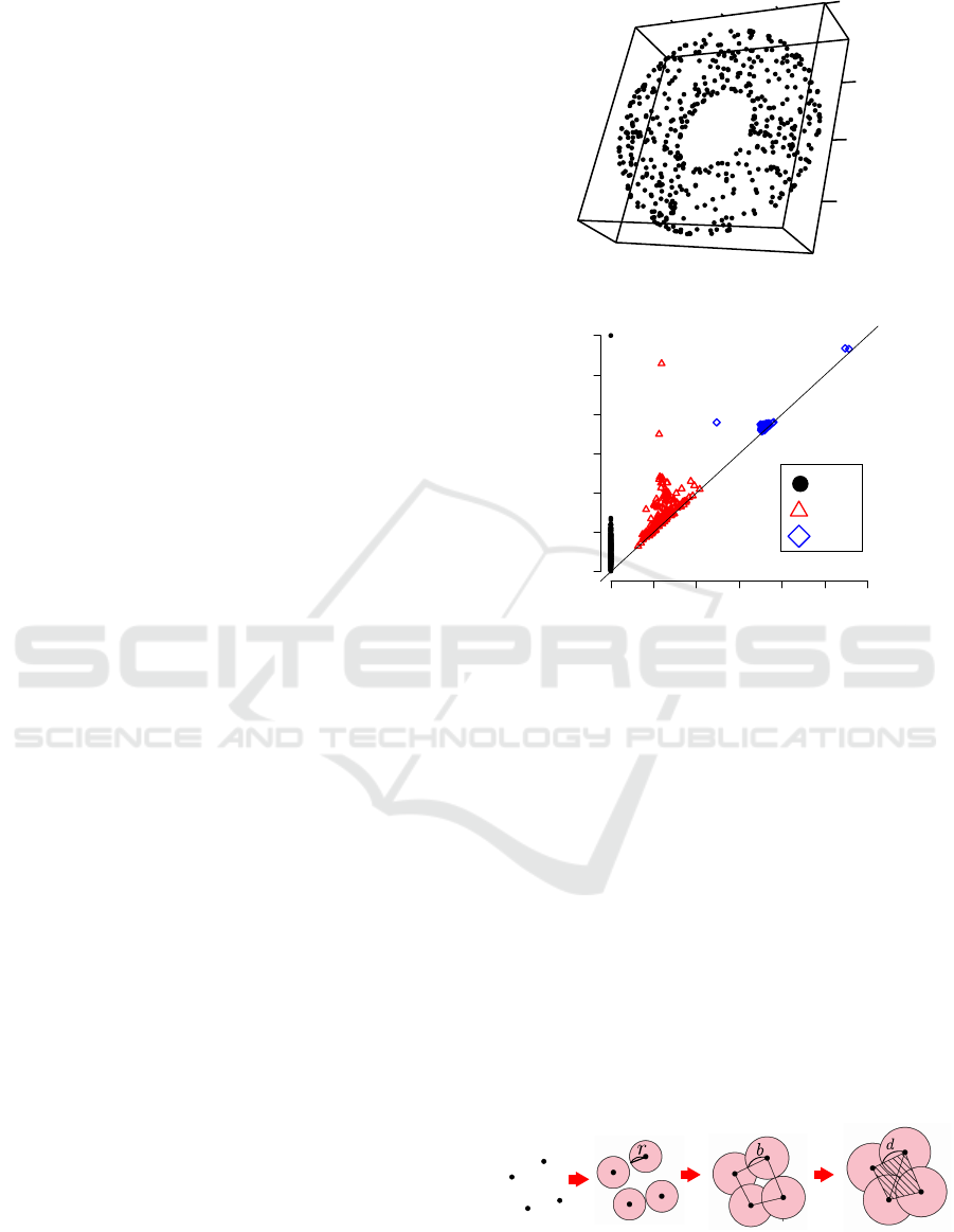
A persistence diagram is a graph that maps (b,d)
as a coordinate (Cohen-Steiner et al., 2007). Figure
2 is the persistence diagram representing the calcula-
tion result of persistent homology of the torus shape
data shown in Figure 1. The difference between birth
and death times (d − b) is called “persistence.” Per-
Figure 1: Torus shape data.
0.0 0.5 1.0 1.5 2.0 2.5 3.0
0.0 0.5 1.0 1.5 2.0 2.5 3.0
Birth
Death
Figure 2: Persistence diagram of torus shape data.
sistence represents the size of holes. In the graph, dis-
tances between each point and the diagonal represents
persistence. The larger the persistence is, the larger
the hole is. Holes with large persistence are usually
considered to be cycles.
The red triangles in Figure 2 indicate 1-
dimensional holes and the blue squares in Figure 2
indicate 2-dimensional holes. The torus that is the un-
derlying manifold of Figure 1 has two 1-dimensional
holes and one 2-dimensional hole. However, many
more holes appear in Figure 2 than there actually are
in the underlying manifold. Noises produced from
gaps among points on the underlying manifold cause
this problem. The method to estimate the number of
cycles in the calculation result of persistent homology
of the data set is required in order to estimate the Betti
numbers of the underlying manifold.
Figure 3: Radius increasing, hole birth and hole death.
ICAART 2020 - 12th International Conference on Agents and Artificial Intelligence
396

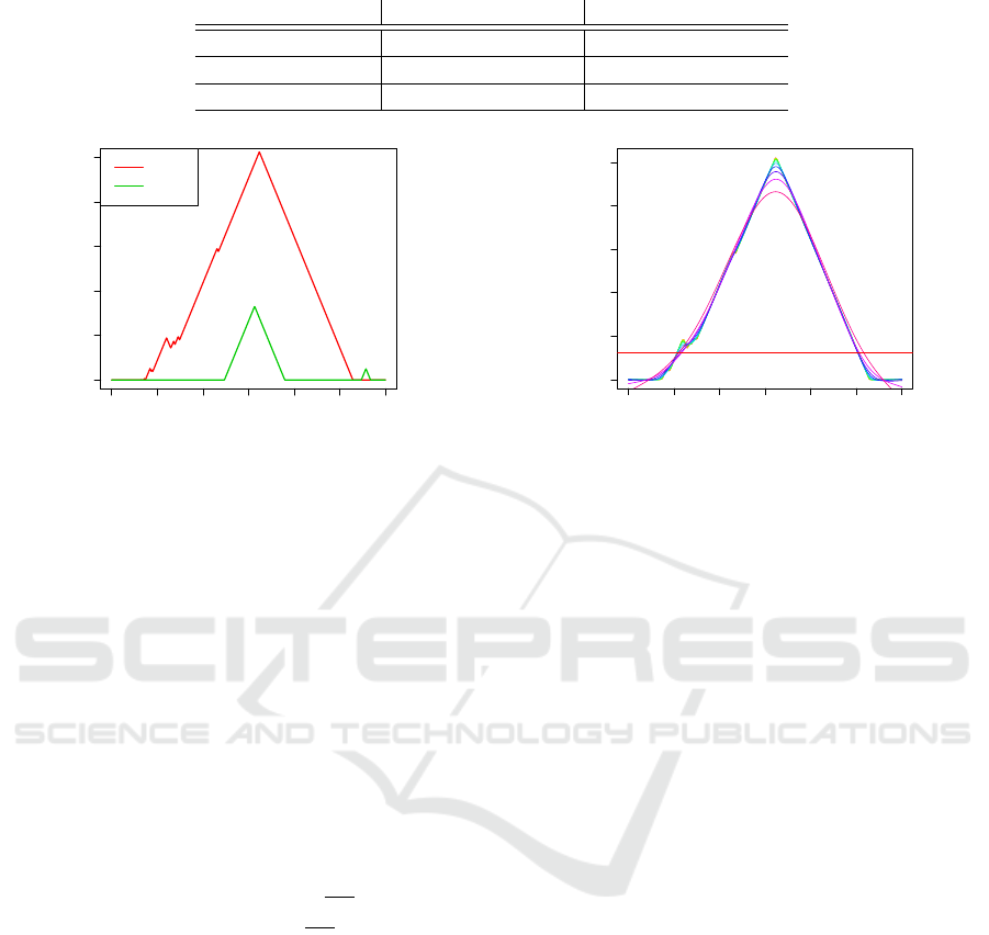
Table 1: The number of holes in topological shapes.
Topological shape 1-dimensional holes 2-dimensional holes
Circle 1 0
Sphere (S
2
) 0 1
Torus (S
1
× S
1
) 2 1
0.0 0.5 1.0 1.5 2.0 2.5 3.0
0.0 0.2 0.4 0.6 0.8 1.0
(Birth + Death) / 2
(Death − Birth) / 2
0.0 0.5 1.0 1.5 2.0 2.5 3.0
0.0 0.2 0.4 0.6 0.8 1.0
(Birth + Death) / 2
(Death − Birth) / 2
dim1
dim2
Figure 4: Persistence landscape of torus shape data.
2.1 Estimating the Betti Numbers by
the Use of Persistent Homology
Analysis
When a data density is high enough, the Betti num-
bers of an underlying manifold is estimated by us-
ing the method proposed by Futagami et al. (2019).
In this section, we describe this conventional method
briefly.
First, to reduce noises, a persistence landscape is
calculated from a persistence diagram. A persistence
landscape is given by mapping each coordinate p =
(b,d) in a persistence diagram D to a piecewise linear
function (Bubenik, 2015), such that
Λ
p
(t) =





t − b t ∈ [b,
b+d
2
]
d − t t ∈ [
b+d
2
,d]
0 otherwise.
(1)
In general, the collection of the largest functions in
Eq.1 is used, such that,
λ(t) = max
p∈D
Λ
p
(t). (2)
Figure 4 is the persistence landscape derived from
Figure 2.
Second, the persistence landscape is smoothed to
determine whether small local maxima on the side of
large local maxima is cycles or noises. Local max-
ima that exist even after high smoothing are consid-
ered to be cycles. Concretely, a persistence land-
scape is smoothed by repeatedly fitting cubic smooth-
ing splines based on B-splines while using various
smoothing parameters. Figure 5 shows the 1-degree
0.0 0.5 1.0 1.5 2.0 2.5 3.0
0.0 0.2 0.4 0.6 0.8 1.0
(Birth + Death) / 2
(Death − Birth) / 2
Figure 5: Smoothed persistence landscape of torus shape
data.
persistence landscapes in Figure 4 smoothed with var-
ious parameters. A red horizontal line in Figure 5 rep-
resents the mean of persistence used as a threshold to
discriminate between cycles and noises. The larger
smoothing parameter is, the smoother a persistence
landscape is.
Third, counting local maxima above the threshold
in each smoothed persistence landscape. The mean
of the number of local maxima above the threshold in
each smoothed persistence landscape is considered to
be the number of cycles in a given data set.
The processes mentioned above are applied to
some subsamples of a given data set. The mean of the
number of cycles in the subsamples is then rounded
off and is considered to be the estimated Betti num-
bers.
2.2 Limit of the Conventional Method
The estimation accuracy of the 2nd Betti numbers us-
ing the method proposed by Futagami et al. (2019)
gets worse as data density decreases. Figure 6 shows
the relationship between data density and the accu-
racy of estimating 2nd Betti numbers. Success rate
represents the rates of data sets whose 2nd Betti num-
bers of their underlying manifold are estimated cor-
rectly among all data sets when using the conven-
tional method. Data density is the number of points
per unit area of the surface of the underlying mani-
fold. The vertical and horizontal axes in Figure 6 rep-
resent the success rate and data density, respectively.
We estimated the 2nd Betti number of data sampled
from the uniform distribution on the torus, as shown
Inferring Underlying Manifold of Low Density Data using Adaptive Interpolation
397

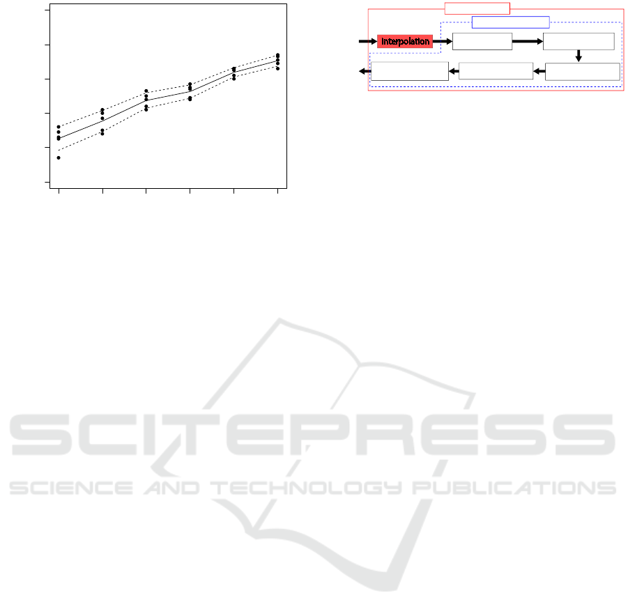
Figure 6: Relationship between data density and success
rates of estimating 2nd Betti number.
in Figure 1, using the conventional method. The ma-
jor radius and the minor radius of the torus were 2.5
and 1, respectively. Then, we calculated the rates of
data sets of which the conventional method estimated
2nd Betti numbers of their underlying manifold cor-
rectly among 100 data sets at once trial. While chang-
ing the number of data points in one data set from
300 to 350 by 10, we conducted this trial five times in
each data density. Each black circle in Figure 6 indi-
cates a success rate for each trial. For example, when
data density is 31/π
2
, that is 310 data points lie on the
torus, the conventional method estimated correctly for
32% of 100 data sets in first trial, and for 35% of 100
data sets in second trial, and for 38% of 100 data sets
in third trial, and for 40% of 100 data sets in fourth
trial, and for 39% of 100 data sets in fifth trial. A
black line and black dashed lines are straight lines
connecting the mean of success rates and the sum or
difference between the mean and standard deviation
of success rates in each data density, respectively.
Figure 6 shows that estimation accuracy gets
worse as data density decreases. When data den-
sity is low, data points is distributed sparsely. There-
fore, being crossed 3-dimensional balls each other
take more time, that is, birth times of 2-dimensional
holes get later, when data density is low. On the other
hand, death times of 2-dimensional holes are about
the same when data density is high. When birth times
is delayed, the persistence of 2-dimensional holes is
smaller and detecting 2-dimensional cycles becomes
more difficult.
Figure 7: Sequence of proposed method.
3 PROPOSED METHOD
3.1 Method to Estimate the Betti
Number using Interpolation
The estimation accuracy of 2nd Betti numbers using
the conventional method gets worse as data density
decreases. Late birth times of 2-dimensional holes
make the persistence of 2-dimensional cycles smaller
and discriminating between cycles and noises more
difficult. Difficulty of detecting cycles causes the poor
estimation accuracy of 2nd Betti numbers. To solve
this problem, we propose a method to estimate 2nd
Betti numbers using interpolation that add points in
sparse areas on an underlying manifold. Using in-
terpolation to make the detection of cycles easier im-
proves the estimation accuracy of 2nd Betti numbers.
We add points close to a tangent space and a point
of tangency in the underlying manifold in our pro-
posed method. According to Zomorodian (2005), in-
tuitively, a manifold is a topological space that locally
looks like R
n
. We approximate a tangent space using
this property that N-dimensional manifold is locally
similar to N-dimensional Euclidean space. Points in a
tiny range on an N-dimensional underlying manifold
are considered to be in an N-dimensional space. Ad-
ditionally, this space is considered to be approximate
to a tangent space. Therefore, we approximate tan-
gent spaces using points in a tiny range on an under-
lying manifold. Adding points in approximated tan-
gent spaces increases data density while retaining the
topological feature of the underlying manifold. In our
proposed method, we use principal component analy-
sis (PCA) to approximate tangent spaces.
However, if too many points are added, the com-
putational time of persistent homology will be too
long to estimate the Betti numbers of an underlying
manifold in most practical applications. Therefore,
we add points only in comparatively sparse areas on
an underlying manifold as much as possible.
The proposed method employs the conventional
method to analyze data set whose density is increased.
Figure 7 shows the sequence of the proposed method.
We describe an interpolation method employed in
the proposed method in Sec.3.2.
ICAART 2020 - 12th International Conference on Agents and Artificial Intelligence
398

Algorithm 1: Interpolating near on Underlying Manifold.
1: Inputs:
X = {x
x
x
1
,··· ,x
x
x
m
} ⊂ R
D
: a input data
M = {1,··· ,m} : indices of X
N : the dimension of underlying manifold of X
K : the number of neighbors
2: Outputs:
ˆ
X : a interpolated point set
3: I ←
/
0
4:
ˆ
X ←
/
0
5: for l ← 1 to m do
6: if l 6∈ I then
7: I ← I ∪ {l}
8: {µ
1
,··· ,µ
K
}
µ
i
∈M
← the indices of the K nearest neighbors of x
x
x
l
l
l
∈ X
9: I ← I ∪ {µ
1
,··· ,µ
K
}
10: {x
x
x
0
0
,x
x
x
0
1
,··· ,x
x
x
0
K
} ← project {x
x
x
l
,x
x
x
µ
1
,··· ,x
x
x
µ
K
} into N-dimensional space using PCA
11: {v
v
v
1
,··· ,v
v
v
p
} ← the vertexes of the Voronoi region of x
x
x
0
0
12: {
ˆ
x
x
x
1
,··· ,
ˆ
x
x
x
p
} ← {
ˆ
x
x
x
i
= U
U
Uv
v
v
i
+ x
x
x
l
}
i=1,···,p
(U
U
U = [u
u
u
1
,··· ,u
u
u
N
] are first to N-th principal vectors derived in
line 10)
13:
ˆ
X ←
ˆ
X ∪ {
ˆ
x
x
x
1
,··· ,
ˆ
x
x
x
p
}
14: end if
15: end for
2
0
-2
x
z
-1
-0.5
0
0.5
1
y
2
0
-2
2
0
-2
x
z
-1
-0.5
0
0.5
1
y
2
0
-2
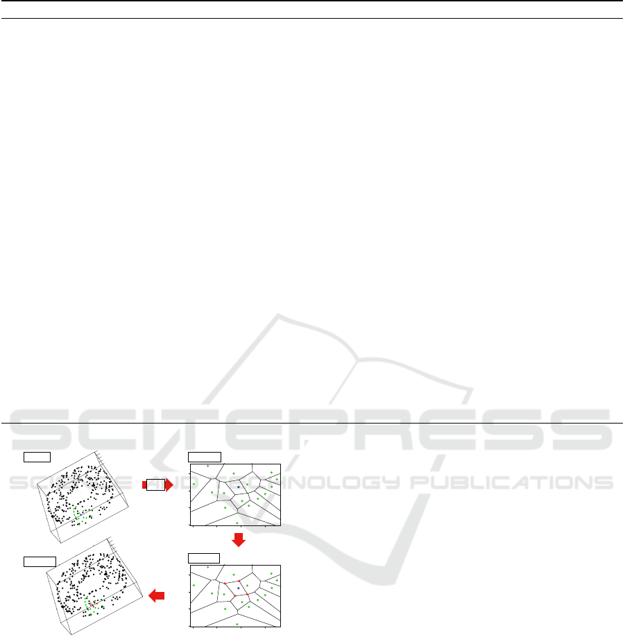
Figure 8: Interpolation that add points close to underly-
ing manifold. ”Line X ” framed by rectangle indicate line
in Algorithm 1. Top Left: Select one point and K near-
est neighbor points. Top Right: Project those points onto
an approximated tangent space using PCA. Bottom Right:
Add points at the vertexes of a Voronoi region. Bottom
Left: Map added points using PCA reconstruction into R
D
,
a space which a given data set belongs to.
3.2 Adding Points into Sparse Areas on
the Underlying Manifold
We describe the interpolation method employed in the
proposed method. Algorithm 1 shows the algorithm
of the interpolation method.
Let X be a point cloud data set of which we want
to estimate the Betti numbers of its underlying mani-
fold. The dimension N of the underlying manifold of
X is determined using the method to estimate the in-
trinsic dimension of X proposed by Hein et al. (Hein
and Audibert, 2005).
Figure 8 show processes in one loop from line 5 to
line 15 in Algorithm 1. ”Line X” framed by rectangle
indicate the line in Algorithm 1. We detail processes
at line 8, 10, 11 and 12 in Algorithm 1 as follows.
Line 8. Select one point x
x
x
l
and K nearest neighbor
points {x
x
x
µ
1
,··· ,x
x
x
µ
K
} of x
x
x
l
. Blue and green points
shown in Figure 8 indicate x
x
x
l
and {x
x
x
µ
1
,··· ,x
x
x
µ
K
},
respectively. Those points are considered to lie
close to a tangent space.
Line 10. Project those points onto an ap-
proximated tangent space using PCA.
Let X
0
= {x
x
x
0
0
,x
x
x
0
1
,··· ,x
x
x
0
k
} be the projected
{x
x
x
l
,x
x
x
µ
1
,··· ,x
x
x
µ
K
}. We put a region for each points
of X
0
, such that
V
i
= {x
x
x
0
∈ R
N
| kx
x
x
0
−x
x
x
0
i
k ≤ kx
x
x
0
−x
x
x
0
j
k, 0 ≤ j ≤ k, j 6= i}
(3)
Those regions V
i
assigned for each x
x
x
0
i
are known
as “Voronoi regions,” and a partitioning of a space
Inferring Underlying Manifold of Low Density Data using Adaptive Interpolation
399

into Voronoi regions is known as a “Voronoi par-
tition.”
Line 11. Add then points at the vertexes {v
v
v
1
,··· ,v
v
v
p
}
of a Voronoi region having x
x
x
0
0
.
Line 12. Lastly, map added points {v
v
v
1
,··· ,v
v
v
p
} using
PCA reconstruction with x
x
x
l
and principal vectors
{u
u
u
1
,··· ,u
u
u
N
} into R
D
, a space which a given data
set belongs to.
In line 12, we use the point x
x
x
l
selected in line 8 in
stead of the mean
¯
x
x
x of x
x
x
l
and K nearest neighbor
points {x
x
x
µ
1
,··· ,x
x
x
µ
K
} for PCA reconstruction. With
x
x
x
l
and principal vectors {u
u
u
1
,··· ,u
u
u
N
}, added points
{v
v
v
1
,··· ,v
v
v
p
} are reconstructed into the space that is
spanned by {u
u
u
1
,··· ,u
u
u
N
} and has x
x
x
l
. Reconstruction
of {v
v
v
1
,··· ,v
v
v
p
} with x
x
x
l
adds points closer to the tan-
gent space that contact with the underlying manifold
at x
x
x
l
than with
¯
x
x
x.
Red points in Figure 8 shows added points
{
ˆ
x
x
x
1
,··· ,
ˆ
x
x
x
p
} using this method. The proposed method
repeats those processes while ensuring that points al-
ready selected as neighbors are not selected again.
Putting points at the vertexes of a Voronoi region
achieves the requisite interpolation that adds points
close to comparatively sparse areas on the underly-
ing manifold. Additionally, once a point has been se-
lected as a neighbor, we do not select it as a candidate
to be the center of neighborhood in order to reduce
the total number of points and any subsequent com-
putational complexity.
4 EXPERIMENT
We estimated the 2nd Betti number of an underlying
manifold of data using the proposed and conventional
methods to confirm that the proposed method esti-
mates more accurately than the conventional method.
Table 2 shows the spec of computer used in the exper-
iment.
4.1 Experiment Settings
We used a point cloud sampled from the uniform dis-
tribution on a torus as one data set in an experiment.
The major radius and the minor radius of the torus
were 2.5 and 1, respectively. We estimated the 2nd
Betti number of the underlying manifold, which is the
torus, using the proposed method. We calculated the
rates of data sets of which the proposed method esti-
mated 2nd Betti numbers of their underlying manifold
correctly among 100 data sets at once trial. While
changing the number of data points in one data set
from 300 to 350 by 10, we conducted this trial five
Table 2: The spec of computer used in the experiment.
OS
Windows Server 2019 Standard
64bit ver.1809
CPU
Intel(R) Xeon(R) Gold 5122 CPU
@ 3.60GHz
RAM 256GB
Figure 9: Torus shape data before interpolating.
times in each data density. Then, we compared the
success rates of estimates given by the proposed and
conventional methods.
4.2 Experiment Results
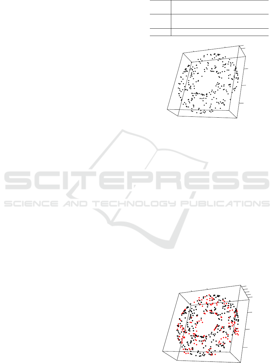
Figure 9 shows one example of the torus shape data
used in the experiment. Additionally, Figure 10
shows torus shape data after applying the interpola-
tion method to the data shown in Figure 9. Red points
in Figure 10 are interpolated points. Comparing Fig-
ure 9 with Figure 10, we find that points are added
close to sparse areas on the torus as intended.
Figure 11 shows the success rates of estimating
2nd Betti numbers using the proposed and conven-
tional methods. Each red and black circle in Figure
11 indicates a success rates of estimating using the
proposed and conventional methods for each trial, re-
spectively. Red and black lines are straight lines con-
Figure 10: Torus shape data after interpolating.
ICAART 2020 - 12th International Conference on Agents and Artificial Intelligence
400

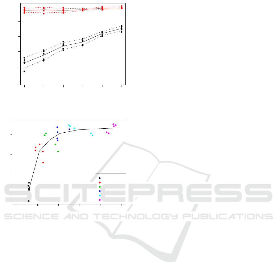
Figure 11: Success rates of estimating 2nd Betti number.
0 5000 10000 15000 20000 25000
0.2 0.4 0.6 0.8
Computational time [sec]
Success Rates
P=0
P=1
P=2
P=3
P=4
all vertexes
300
300
300
300
300
333.41
333.55
333.42
333.38
333.24
366.8
367.07
366.81
366.72
366.47
399.97
400.42
399.92
399.76
399.41
431.83
432.21
431.77
431.34
430.83
494.32
494.02
493.09
489.97
489.81
Figure 12: Relationship between computational time and
success rate.
necting the mean of success rates by the proposed and
conventional methods, respectively. Red and black
dashed lines are also straight lines connecting the sum
or difference between the mean and standard devia-
tion of success rates by the proposed and conventional
methods in each data density, respectively. Figure 11
shows that the proposed method estimated much more
accurately than the conventional method.
We confirmed that the proposed method estimated
2nd Betti number much more accurately than the con-
ventional method based on the experimental result.
The proposed method is effective to estimate 2nd
Betti numbers of the underlying manifold of low den-
sity data.
4.3 Trade-off between Accuracy and
Computational Time
We confirm relationship between the accuracy of es-
timating 2nd Betti numbers and computational times.
We examined estimation accuracy and computational
times when changing the number of points added to
toruses that were used in the experiment and had 300
points. In order to change the number of added points,
we added points at P vertexes of Voronoi region hav-
ing x
l
in descending order of distance between x
l
and
vertexes in the interpolation method employed in the
proposed method. We used 1, 2, 3 and 4 for P. We
calculated the rates of data sets of which the proposed
method estimated 2nd Betti numbers of their under-
lying manifold correctly among 100 data sets at once
trial. While changing P, we conducted this trial five
times in each P.
Figure 12 shows relationship between the accu-
racy of estimating 2nd Betti numbers and compu-
tational time when changing the number of added
points. The vertical and horizontal axes in Figure
12 represent the rates of data sets estimated correctly
among 100 data sets and computational times to esti-
mate 2nd Betti numbers of 100 data sets, respectively.
Red, green, blue and light blue circles in Figure 12 in-
dicate the results when P is 1, 2, 3 and 4, respectively.
Black circles indicate the results when P = 0, that is
when using the conventional method. Purple circles
indicate the results when added points at all vertexes
of Voronoi region. The numbers beside circles indi-
cate the mean of the numbers of points of data sets in
each trial. Black straight line conects the mean of the
results in each P.
Figure 12 shows that the computational times in-
crease as added points increase. The proposed method
estimated 2nd Betti numbers more accurately than the
conventional method. On the other hand, the pro-
posed method costed more computational time to es-
timate than the conventional method. The trade-off
between accuracy and computational times as shown
in Figure 12 occurs when using the proposed method.
5 CONCLUSION
In this study, we propose the method to estimate the
2nd Betti numbers of the underlying manifold us-
ing the interpolation method that adds points close
to comparatively sparse areas in the underlying man-
ifold. Then, we confirm that the proposed method es-
timated 2nd Betti number of the underlying manifold
more accurately than the conventional method. Con-
sequently, we confirm that our proposed method is ef-
fective for estimating 2nd Betti numbers of the under-
lying manifold even when data density is in the range
in which the conventional method often estimates 2nd
Betti number incorrectly. Adding points close to the
underlying manifold enables the proposed method to
estimate 2nd Betti number of the underlying manifold
Inferring Underlying Manifold of Low Density Data using Adaptive Interpolation
401

with greater accuracy.
We would like to confirm the effectiveness of the
proposed method for other manifolds in future re-
search. We also would like to create a method to in-
terpolate with fewer errors.
REFERENCES
Bishop, C. M. (2006). Pattern Recognition and Ma-
chine Learning (Information Science and Statistics).
Springer-Verlag, Berlin, Heidelberg.
Bubenik, P. (2015). Statistical topological data analysis
using persistence landscapes. Journal of Machine
Learning Research, 16:77–102.
Cohen-Steiner, D., Edelsbrunner, H., and Harer, J. (2007).
Stability of persistence diagrams. Discrete & Compu-
tational Geometry, 37(1):103–120.
Edelsbrunner, H. and Harer, J. (2008). Persistent homology
- a survey. Surveys on Discrete and Computational
Geometry, 453:257–282.
Futagami, R. and Shibuya, T. (2016). A method deciding
topological relationship for self-organizing maps by
persistent homology analysis. In 2016 55th Annual
Conference of the Society of Instrument and Control
Engineers of Japan (SICE), pages 1064–1069.
Futagami, R., Yamada, N., and Shibuya, T. (2019). Infer-
ring underlying manifold of data by the use of persis-
tent homology analysis. In Marfil, R., Calder
´
on, M.,
D
´
ıaz del R
´
ıo, F., Real, P., and Bandera, A., editors,
Computational Topology in Image Context, pages 40–
53, Cham. Springer International Publishing.
Hein, M. and Audibert, J.-Y. (2005). Intrinsic dimensional-
ity estimation of submanifolds in rd. In Proceedings of
the 22nd International Conference on Machine Learn-
ing, ICML ’05, pages 289–296, New York, NY, USA.
ACM.
Zomorodian, A. and Carlsson, G. (2005). Computing per-
sistent homology. Discrete & Computational Geome-
try, 33(2):249–274.
Zomorodian, A. J. (2005). Topology for Computing. Cam-
bridge Monographs on Applied and Computational
Mathematics. Cambridge University Press.
ICAART 2020 - 12th International Conference on Agents and Artificial Intelligence
402