Peer-to-peer Energy Trading for Smart Energy Communities
Roman Denysiuk
2,∗ a
, Fabio Lilliu
1,∗ b
, Diego Reforgiato Recupero
1,∗ c
and Meritxell Vinyals
2,∗
1
Department of Mathematics and Computer Science, University of Cagliari, Via Ospedale 72, Cagliari, Italy
2
CEA, LIST, 91191 Gif-sur-Yvette, France
∗
These authors contributed equally to this work
Keywords:
Renewable Energies Incentive Systems, Smart Grid, Game Theory, Peer-to-peer Energy Trading.
Abstract:
Local energy communities (LECs) comprise prosumers cooperating for the satisfaction of their energy needs.
Prosumers are community members that can both produce and consume energy. LECs facilitate the integration
of renewables and provide the potential for reducing energy costs. Peer-to-peer (P2P) energy trading allows
direct energy exchange between members of a local energy community. The surplus of energy from renew-
ables is traded to meet a local consumption demand so that costs and revenues stay within community avoiding
transmission losses and stress on the grid. This study presents a design of the peer-to-peer market for local
energy communities where prosumers are rational and self-interested agents acting selfishly in an attempt to
optimize their trades. The market design aims to ensure self-consumption of locally produced energy and pro-
vides incentives for balancing supply and demand within community. The proposed design is investigated in
comparison with existing ones using theoretical analysis and simulations. The obtained results are promising
and reveal advantageous properties of the proposed P2P energy trading.
1 INTRODUCTION
Nowadays, the topics of energy and climate policies
are crucial, and require a transition for energy systems
from exhaustible energy sources, such as fossil and
nuclear, to renewables (e.g. wind and solar). About
this, several policies have been made in order to sup-
port installation and employment of renewable energy
sources (RES). These policies reward RES produc-
ers for the excess of energy they export to the grid,
for example by paying them money for unit of en-
ergy exported or by providing them energy at no cost
later, so that they are repaid for their RES investment.
These policies have been effective for increasing the
share of energy generated from RES, which in 2016
already represented 30% of total energy generated in
Europe
1
; however, the employment of this type of
energy comes with stability problems to the grid (Mi-
haylov et al., 2019; Commission, 2013), and support
policies are unable to solve this at the moment, so this
limits their effectiveness. More precisely, renewable
a
https://orcid.org/0000-0002-6847-8313
b
https://orcid.org/0000-0003-1140-4433
c
https://orcid.org/0000-0001-8646-6183
1
http://www.eea.europa.eu/data-and-maps/indicators/
overview-of-the-electricity-production-2/assessment
energy production is difficult to control, and for this
reason production usually does not match consump-
tion.
In order to face these issues, in these years
there have been new proposals for incentive mecha-
nisms (Ilic et al., 2012; Mihaylov et al., 2014; Kok
et al., 2005; Capodieci et al., 2011). The key feature
of these mechanisms is building the payment support
functions for producers and consumers in such a way
that, at every moment, energy consumption is encour-
aged to match energy production.
Some of these mechanisms use market-based ap-
proaches (Ilic et al., 2012; Kok et al., 2005), which
consider a local market where prosumers sell the en-
ergy they produce and consumers buy it. Another
work by (Mihaylov et al., 2014) proposes a mecha-
nism called NRG-X-Change, which does not rely on
an energy market, as locally produced renewable en-
ergy is simply injected into the grid and taken by con-
sumers. Unlike traditional support policies, the NRG-
X-Change mechanism offers incentives not only for
producers but also consumers, depending on their
contribution to the local energy balance.
The most prominent feature of NRG-X-Change
is the employment of NRGcoin, a virtual currency
whose exploitation offers some relevant benefits to
40
Denysiuk, R., Lilliu, F., Recupero, D. and Vinyals, M.
Peer-to-peer Energy Trading for Smart Energy Communities.
DOI: 10.5220/0008915400400049
In Proceedings of the 12th International Conference on Agents and Artificial Intelligence (ICAART 2020) - Volume 1, pages 40-49
ISBN: 978-989-758-395-7; ISSN: 2184-433X
Copyright
c
 2022 by SCITEPRESS – Science and Technology Publications, Lda. All rights reserved

energy trading. However, there are some important
factors not taken into account by this mechanism,
such as energy self-consumption and the management
of congestion. More precisely, we want to ensure that
prosumers always consume their produced energy be-
fore selling or buying the excess energy they produce
or need. In other words, we want to actively discour-
age scenarios where the energy consumption or pro-
duction is excessive. Therefore, the purpose of this
work is to create a new incentive mechanism based
on NRG-X-Change and the use of NRGcoin using as a
baseline the works in (Mihaylov et al., 2014) and (Lil-
liu et al., 2019b), but further improving the critical
points of the mechanism and studying its behavior in
a context with selfish agents. The contributions of this
paper are therefore the following:
• We analyze the NRG-X-Change project and iden-
tify its main issues (import and export price func-
tions) and the situations where they appear;
• We design new import and export price functions
that can work better within the NRG-X-Change
mechanism by exploiting known results in game
theory about Nash Equilibria, and provide theo-
retical background on those;
• We demonstrate the validity of our proposed func-
tions through mathematical proof, and carry out
an experimental evaluation on real data from a
grid in Cardiff that measured the efficiency of our
proposed functions.
The remainder of the paper is structured as fol-
lows. Section 2 describes the literature related to
our work. Section 3 formulates the game theoretical
model, and in Section 4 we present the baseline we
work on top, and how we want to achieve the objec-
tives of this paper. Section 5 validates our theoretical
results and quantifies the efficiency of the described
mechanisms via simulations using real data from a
grid in Cardiff (UK). Finally Section 6 concludes the
paper and describes possible future developments.
2 RELATED WORK
Although the NRG-X-Change mechanism has not yet
been implemented in actual grids, there are some
works in which it has been described in detail. The
most important one is from (Mihaylov et al., 2014),
where the authors explain the advantages of using
a digital currency and the interactions between grid
users, with or without outside parties. Also, (Mi-
haylov et al., 2015) created a scenario simulating a
local grid, showing how NRG-X-Change performs in
a realistic environment.
A survey on incentive mechanisms has been done
by (Mihaylov et al., 2019), where issues about net me-
tering and feed-in tariffs are discussed, such as over-
consumption in some periods of the year, overpay-
ment for the energy provider, and underpayment to
energy producers. In that work, there is a comparison
of some new support mechanisms which aim to solve
these problems. One of them is the auction-based
mechanism Nobel (Ilic et al., 2012), which trades
energy at a local level based on the stock exchange
model. Another mechanism is PowerMatcher (Kok
et al., 2005), which is based on a market structure
regulated by software agents balancing demand and
supply in a tree-shaped hierarchical structure, and are
called SD-matchers. There is also a work proposed
by (Capodieci et al., 2011), which is a negotiation-
based mechanism where prosumers compete with en-
ergy generating companies (Gencos) for selling en-
ergy, and negotiate the price with buyers. It is then
shown how this mechanism affects the energy price,
and also what happens with the implementation of
a learning strategy for the buyers. However, all
these above-cited works focus on market mechanisms
which require final prosumers to get involved into
complex bidding processes.
Literature on employment of game theory for the
smart grid context is extensive. (Saad et al., 2012)
present a survey which describes comprehensively
how game theory methods have been used for smart
grid. The work done by (Rad et al., 2010) is prob-
ably one of the closest to the work we propose here
in terms of employment of game theory, although its
focus is mainly devoted to manage demand response
whereas ours is on the incentive mechanism. The
game theory usage done by (Nguyen et al., 2012)
and (Soliman and Leon-Garcia, 2014) has also been
of inspiration for us, since the model we will propose
in this work has been heavily influenced by their game
theory modeling in the smart grid context. The work
from (Loni and Parand, 2017) contains another survey
describing the use of game theory for smart grid, al-
though it focuses on collaborative games, whereas our
work describes mainly a situation where each agent is
selfish.
3 MODELIZATION OF THE
PROBLEM
In this section the modelization of the problem will
be discussed. We built a model from a game theory
perspective in order to explain the effect of the incen-
tive mechanism on the agents. Our construction was
inspired by (Nguyen et al., 2012) and (Soliman and
Peer-to-peer Energy Trading for Smart Energy Communities
41

Leon-Garcia, 2014).
3.1 Game Theory Approach to Our
Smart Grid Problems
First, we introduce our notation for game theory. We
define a game G = (U,S,Q) in the following way:
• U = {U
1
,...,U
N
} is the set of players.
• S = {S
1
,...,S
N
}, where for any i ∈ {1,...,N}, S
i
is the set of player U
i
’s strategies.
• Q = {q
1
,...,q
N
}, where for any i ∈ {1,...,N},
q
i
:
N
∏
j=1
S
j
→ R is the payoff function for player
U
i
.
Let us consider a grid with N users: we will now
define a game on it. The players are the grid users,
which will thus be denoted as U
i
, for i ∈{1,...,N}. In
what follows we describe the users’ payoff functions
and the strategies they are allowed to choose.
For each user U
i
, we define a vector c
i
which in-
dicates the energy consumption of U
i
, and a vector p
i
which indicates the energy production of U
i
. The size
of these vectors is the number of intervals in which the
considered time horizon is divided: for example, in a
scenario with a 24 hour time horizon with 15 minutes
intervals, the size of c
i
and p
i
is 96. Each component
of both c
i
and p
i
is a non-negative real number. We
will denote this number of time intervals as T .
One important consideration has to be made about
the values of c
i
and p
i
: in this work we assume that
each user self-consumes all the energy she
2
needs
before exporting it or imports the extra energy she
needs, and the values of c
i
and p
i
are considered after
self-consumption is taken into account. This, in for-
mal terms, denoting as c
i
(t) the t−th element of c
i
, is
written as
c
i
(t) ·p
i
(t) = 0 ∀t ∈ 1, . . . , T (1)
for each i ∈{1,...,N}. Of course, if U
i
is a consumer
which does not produce energy, p
i
is the zero vector.
Later in this work, we will ensure that all the payment
functions we propose actively encourage energy pro-
ducers to self-consume their produced energy.
Now, we can define the utility function q
i
for each
grid user as the sum of the utility in the different time
intervals, namely:
q
i
=
T
∑
t=1
q
i
(t) (2)
where the utility of a user U
i
at time interval t is de-
fined as:
q
i
(t) = g(p
i
(t),t
p
,t
c
) −h(c
i
(t),t
p
,t
c
). (3)
2
from now on, this is to be read as he/she.
where g and h are two pre-determined functions with
the property that g(0,a, b) = h(0,a,b) = 0 for every
a,b ∈ R, and represent respectively the reward for
the energy produced, and the cost for the energy con-
sumed. Fixed a time unit t, the aforementioned quan-
tities t
p
and t
c
are defined as
t
p
=
N
∑
i=1
p
i
(t)
t
c
=
N
∑
i=1
c
i
(t)
(4)
and represent the total production and the total con-
sumption through the grid at that given time. In par-
ticular, at a given time t, t
p
depends on every p
i
(t) and
t
c
on every c
i
(t).
The formulation of costs and rewards based on
functions which take into account the total production
and the total consumption at a certain time has been
inspired by (Mihaylov et al., 2014): this has been the
work we used as baseline to build on top.
Next, we show the possible strategies for the play-
ers. More precisely, how the loads can be modeled
in our scheme. An example of this has been seen in
the work from (Soliman and Leon-Garcia, 2014). In
the following we will indicate the loads that we have
taken into consideration for our work.
• Production: This is p
i
. It represents the energy
production of the user U
i
, and it is a fixed vector
unless the energy production is somehow modu-
lable, which is not our case.
• Fixed Consumption: This is a fixed vector f
i
. It
represents the fixed part of the energy consump-
tion of the user U
i
. In this work it will be treated
as a known vector, although it has to be forecast
and may present uncertainty: a possible approach
to this issue can be the one used by (Lilliu et al.,
2019a), which treat the components of the vector
as probability distributions.
• Shiftable Load: This is a vector h
i
j
, which rep-
resents a consumption load of user U
i
which can
be shifted in time. The user can control how many
time units this vector can be shifted by, although
sometimes they have restrictions on this. Given
the vector h
i
j
, the notation r
k
(h
i
j
) will indicate
that vector shifted by k places. In other words, r
k
indicates the rotation by k places: if k = 0 there is
no rotation, therefore r
0
(h
i
j
) = h
i
j
.
Thus, if a user has n shiftable loads {h
i
1
,...,h
i
n
}, and
decides to shift each h
i
j
by a quantity k
j
, we have
c
i
= f
i
+
n
∑
j=1
r
k
j
(h
i
j
). (5)
ICAART 2020 - 12th International Conference on Agents and Artificial Intelligence
42

The set of possible strategies of U
i
is then the set of
all her possible vectors p
i
and c
i
, depending on how
the loads are shifted.
4 PEER-TO-PEER MARKET
DESIGN
This section presents the proposed peer-to-peer mar-
ket for energy trading.
4.1 Purpose
The goal of this paper is to modelize an incentive
mechanism for renewable energy, using as a baseline
the NRG-X-Change (Mihaylov et al., 2014) mecha-
nism, but improving some of its critical points. More
precisely, these points are:
1. Ensuring that prosumers are not incentivized to
curtail their own energy production, unless this is
necessary for the grid stability.
2. Taking into account the possibility of a conges-
tion, and actively attempting to prevent it.
3. Encouraging prosumers to self-consume the en-
ergy they produce before selling, or before buying
from the grid the excess energy they need.
4. Analyzing the behavior of the users if they mod-
ulate selfishly their production and consumption,
and ensure that they reach an equilibrium.
in their work, (Lilliu et al., 2019b) have addressed
the first three points by creating functions which de-
scribe rewards for energy production and costs for
energy consumption respectively. The scope of this
work is to create new functions which address all of
the four points mentioned above.
4.2 The NRG-X-Change Incentive
Mechanism
First, we describe the baseline on which we have built
our work. The first thing to be described is NRG-X-
Change: it is an incentive mechanism based on the
usage of a virtual currency.(Mihaylov et al., 2014)
Its functioning is described as follows. At each
time unit, grid users may produce and consume en-
ergy. Suppose that at a certain time unit, the user
U
i
produces energy and injects an amount x of en-
ergy into the grid. The user is then rewarded a certain
amount of NRGcoins for the energy produced. This
amount is regulated by a function, which is defined as
g(x,t
p
,t
c
) = x ·
q
e
(t
p
−t
c
)
2
a
(6)
where q and a are two parameters, the first indicating
the maximum value of the tariff, the second calibrat-
ing the function.
Similarly, if at a certain time unit the user U
i
con-
sumes an amount y of energy from the grid, she will
pay a certain amount of NRGcoins for that. This
amount is regulated by a function, which is defined
as
h(y,t
p
,t
c
) = y ·
r ·t
c
t
c
+t
p
(7)
where r is a parameter which determines the maxi-
mum possible value of the tariff.
These tariffs have been chosen in order to regu-
late consumption, so that users are encouraged to con-
sume energy when local production is higher than lo-
cal consumption, and discouraged to consume when
local production is lower. Also, production is re-
warded more when local production and consumption
are similar, in order to encourage balance between
them.
However, this system has several flaws, which the
paper from (Lilliu et al., 2019b) has pointed out and
addressed by creating one new function for reward-
ing energy production and one for determining costs
for energy consumption. These functions will be de-
scribed now.
We indicate with t
p
−i
and t
c
−i
the values of t
p
and
t
c
if x and y are both zero. In other words,
t
−i
p
=
∑
j6=i
p
j
(t)
t
−i
c
=
∑
j6=i
c
j
(t)
(8)
The new selling function g is defined as
g(x,t
p
,t
c
) =P
max
·

g
1
(t(x,t
−i
p
,t
−i
c
))−
g
1
(t(0,t
−i
p
,t
−i
c
))

−P(x,t
−i
p
,t
−i
c
)
(9)
where P(x,t
−i
p
,t
−i
c
) is a penalty term, which is positive
if t
−i
p
and t
−i
c
are such that a congestion will happen
(i.e. |t
−i
p
+ x −t
−i
c
|> B), and zero otherwise, and P
max
is a scaling factor used to determine the tariff. In this
definition, g
1
is a function defined as
g
1
(t) =







0 i f t ≤ 0
1
1+e
2t−1
t
2
−t
i f t ∈ (0,1)
1 i f t ≥ 1
(10)
which determines the shape, and t is a function de-
fined as
t(x,t
−i
p
,t
−i
c
) =
t
−i
p
+ x −t
−i
c
2B
+
1
2
(11)
where B is a constant, depending on the maximum
difference between t
−i
p
and t
−i
c
which will not corre-
spond to a congestion.
Peer-to-peer Energy Trading for Smart Energy Communities
43

The new buying function h is defined as
h(y,t
−i
c
,t
−i
p
) =
Q
max
·h
1
(
t
−i
c
+ y −t
−i
p
B
+ 1) ·y + P(y,t
−i
c
,t
−i
p
).
(12)
Q
max
is a parameter used in order to determine the
tariff value, corresponding to the maximum cost per
unit of energy; B is a parameter corresponding to the
congestion threshold like in the definition of Eq. (11),
and P(x,t
−i
c
,t
−i
p
) is a penalty factor which is zero for
t
−i
c
+ y −t
−i
p
< B and positive otherwise.
In the above definition, the function h
1
is defined
as:
h
1
(t) =









0 i f t ≤ 0
√
t i f t ∈ (0,1]
2 −
√
2 −t i f t ∈ [1,2)
2 i f t ≥ 2.
(13)
These new functions solve many of the issues of the
original NRG-X-Change work, but still have to be an-
alyzed from a game theoretical perspective. In order
to do so, we have to use the model defined in Sec-
tion 3 and analyze the behavior of the players with
the payoff functions relative to each system.
For the original NRG-X-Change work, it is not
difficult to write q
i
(t): using Eq. 3, it can be written
as
q
i
(t) = x ·
q
e
(t
p
−t
c
)
2
a
if y = 0
q
i
(t) = −y ·
r ·t
c
t
c
+t
p
if x = 0
(14)
keeping in mind that either x or y is equal to zero, as
seen in Eq. 1.
As mentioned by (Lilliu et al., 2019b) the expres-
sion for q
i
is more complicated to write, although
it may be simplified if we consider different cases.
Since at least one between x and y is equal to zero,
substituting Eq. (10) and (11) in Eq. (9) and Eq. (13)
in Eq. (12):
• If y = 0, i.e. the user’s production is greater than
the user’s consumption, we have
q
i
(t) =
P
max
1 + e
2
t
−i
p
+x−t
−i
c
B

t
−i
p
+x−t
−i
c
B

2
−
1
4
−
P
max
1 + e
2
t
−i
p
−t
−i
c
B

t
−i
p
−t
−i
c
B

2
−
1
4
(15)
• If x = 0, i.e. the user’s consumption is greater than
the user’s production, we have
– If t
−i
p
> t
−i
c
,
q
i
(t) = −y ·Q
max
·
s
t
−i
c
+ y −t
−i
p
B
+ 1 (16)
– If t
−i
p
< t
−i
c
+ y,
q
i
(t) = −y ·Q
max
·

2 −
s
1 −
t
−i
c
+ y −t
−i
p
B

(17)
An important remark has to be made: since the
production suffers from no curtailment, but x is the
value of production minus consumption, a prosumer
may change this value by changing her consumption.
4.3 New Proposals
Among the points listed in Section 4.1, the fourth is
the one which still has to be solved. Basically we want
to check whether a Nash Equilibrium (NE) exists for
the previously defined incentive systems, and in case
it does not, to create new possible selling and buying
functions which guarantee the existence of a NE while
fulfilling the first three points listed in Section 4.1.
For the first two systems, our strategy has been the
following: first, create a simulation of the described
game in order to see empirically whether a NE exists
or not, and if the answer was positive, find a mathe-
matical proof of its existence. As we will see in Sec-
tion 5, these functions do not guarantee the existence
of a NE.
We wanted to create selling and buying functions
which guarantee the existence of a NE in the game we
described. For this, we exploited a well-known result:
a game with a concave payoff function admits a pure
NE (Nguyen et al., 2012). So, if we can create a con-
cave selling function and a convex buying function,
the utility function defined in Eq. 3 will be concave
and the theorem proven by (Rosen, 1965) will guar-
antee the existence of a pure NE.
However, this may create conflicts with the other
points, in particular with the condition for avoiding
curtailment and the self-consumption condition. For
the former, it is enough to ensure that the selling func-
tion g is a monotonic function with respect to x. In
order to check the latter, however, we want to see that
the following condition
g(x,t
p
,t
c
) < h(x,t
p
,t
c
) (18)
holds for each x > 0 and for each t
p
,t
c
≥ 0.
Some ideas for functions that respect the above
constraints may be the following. We will denote
Z = t
−i
p
−t
−i
c
+ B. (19)
• For the selling function g:
– [Logarithm] One idea may be to base the func-
tion on logarithm. In this case, the function can
be
g(x,t
p
,t
c
) = k
1
·

ln
x + Z + a
1
Z + a
1

(20)
ICAART 2020 - 12th International Conference on Agents and Artificial Intelligence
44

where a
1
and k
1
are parameters, and a
1
> 0.
– [Square root] Another idea may be to use the
square root function as a base. In this case, a
possible candidate is
g(x,t
p
,t
c
) = k
1
·(
√
x + Z + a
1
−
√
Z + a
1
)
(21)
where a
1
and k
1
are parameters, and a
1
> 0.
• For the buying function h:
– [Quadratic] One possibility is to use the
quadratic function. In this case, a candidate
may be
h(y,t
p
,t
c
) = k
2
·((y −Z + a
2
)
2
−(a
2
−Z)
2
)
(22)
where a
2
and k
2
are parameters, and a
2
> 2B.
– [Square root] Another possibility for this may
be the negative square root function. In this
case, our function may have the following
form:
h(y,t
p
,t
c
) = k
2
·(
√
Z + a
2
−
p
Z + a
2
−y)
(23)
where a
2
and k
2
are parameters, and a
2
> 0.
To each of the proposed functions a term P has to
be added. For selling functions, P is a function deter-
mined by x, t
p
and t
c
such that its value is zero unless
t
p
−t
c
> B, in which case it is negative. For buying
functions, P depends on y, t
p
and t
c
and its value is
zero unless t
c
−t
p
> B, in which case it is positive. In
other words, P is a penalty term which punishes over-
production/overconsumption when it causes a con-
gestion. Notice that, with the used notation, a con-
gestion occurs if and only if Z /∈ (0,2B).
These functions have been designed to have a cer-
tain behavior in relation to the variable Z. When local
energy consumption is higher than local energy pro-
duction, the energy generated by producers is valu-
able since it helps covering the consumption needs of
the community: in this case the selling functions as-
sume higher values, and consequently producers are
paid more for the energy they produce. On the other
hand, when local energy production is higher than lo-
cal energy consumption, the surplus energy injected
by the producers is not needed by the consumers, so
the selling functions assume lower values and energy
producers are paid less. As far as the buying func-
tions are concerned, when local energy consumption
is higher than local energy production we want to dis-
courage consumers from consuming energy, since en-
ergy has to be bought from outside the community:
for this reason, buying functions assume higher val-
ues and the price for buying energy is higher for con-
sumers. Conversely, when local energy consumption
is lower than local energy production, we want to
encourage consumers to consume energy, since they
would use the energy generated by the producers: for
this reason, buying functions assume lower values and
consequently energy costs less for the consumers.
It is not difficult to check that the proposed sell-
ing functions are monotonic: the more energy a user
produces, the more she is paid for. For this reason
the user is discouraged from curtailing her own en-
ergy production, since curtailment would decrease her
profits. The only exception is the case of congestion
for overproduction, where the penalty term discour-
ages producers from generating energy by lowering
their profits. This is the first condition described at
the beginning of Section 4.1, which is then respected
by our functions: we want to ensure that the func-
tions we create satisfy all of them. The second con-
dition that has to be fulfilled is the fact that both sell-
ing and buying functions actively consider the possi-
bility of congestion: since the functions we are cre-
ating have a penalty term for congestion, they fulfill
this condition. We will prove in Section 5.1 that the
proposed functions respect also the third condition,
while the last condition holds because of the theorem
proven by (Rosen, 1965). This theorem implies that
our game guarantees the existence of a Nash Equilib-
rium if the payoff functions are concave; it is easy to
check that this is true from Eq. 3, since the proposed
selling functions are concave and the proposed buying
functions are convex.
5 SIMULATIONS AND RESULTS
This section is divided in two parts. In Section 5.1
the constraint for encouraging self-consumption due
to pricing is proven to hold for the newly proposed
functions, while in Section 5.2 it is proven that the
baseline functions do not guarantee the existence of a
NE, while the new proposed functions always reach a
NE as expected from the theoretical results.
5.1 Parameter Settings
The goal of this section is to verify that the functions
proposed in this work respect the self-consumption
condition, which is expressed in Eq. 18. We will ana-
lyze the behavior of the functions, and check if there
is a choice for the parameters such that the condition
is fulfilled.
Peer-to-peer Energy Trading for Smart Energy Communities
45

5.1.1 Candidate 1: Logarithm Selling,
Quadratic Buying
This is the case where the selling function g is the
one described in Eq. 20, while the proposed buying
function h is the one described in Eq. 22.
We want to check that Eq. 18 holds for some
choice of the parameters of these two functions. By
rewriting this condition with the two functions, we
want to prove that there is a choice for the parame-
ters k
1
, a
1
, k
2
and a
2
such that
k
1
·

ln
x + Z + a
1
Z + a
1

< k
2
·

(x−Z +a
2
)
2
−(a
2
−Z)
2

holds for each x > 0 and Z ∈(0, 2B).
Lemma 1. For each x > 0, Z > 0, a
1
≥ 1 and a
2
≥
2B + 1, and choosing k
1
= k
2
> 0, the inequality
ln

1 +
x
Z + a
1

k
1
< k
2
·x ·(x −2Z + 2a
2
) (24)
holds.
Proof. Considering the exponent, Eq. 24 becomes

1 +
x
Z + a
1

k
1
< e
k
2
·x·(x−2Z+2a
2
)
Since k
1
= k
2
, we can remove the equal exponents and
the inequality that we want to prove becomes
1 +
x
Z + a
1
< e
x·(x−2Z+2a
2
)
Thus, exploiting the properties a
1
≥ 1 and a
2
≥ 2B +
1, the chain of inequalities
1+
x
Z + a
1
≤1+
x
Z + 1
< 1+x < e
x
2
+x
≤e
x·(x−2Z+2a
2
)
completes the proof, since it holds for every value of
x > 0 and Z ∈(0, 2B).
Proposition 1. The function defined in Eq. 20 with
a
1
= 1, together with the function defined in Eq. 22
with a
2
= 2B + 1, satisfies the self-consumption con-
dition defined in Eq. 18 if k
1
= k
2
> 0.
Proof. Thanks to Lemma 1, with the aforementioned
choice of parameters, the chain of inequalities
k
1
·ln

x + Z + a
1
Z + a
1

= ln

x + Z + a
1
Z + a
1

k
1
=
= ln

1 +
x
Z + a
1

k
1
< k
2
·x ·(x −2Z + 2a
2
) =
k
2
·

(x −Z + a
2
)
2
−(a
2
−Z)
2

.
holds for each x > 0, Z ∈(0, 2B).
5.1.2 Candidate 2: Square Root Selling,
Negative Square Root Buying
This is the case where the selling function g is the
one described in Eq. 21, while the proposed buying
function h is the one described in Eq. 23.
Proposition 2. There is a choice for the parameters
k
1
and a
1
for the selling function defined in Eq. 21,
and for the parameters k
2
and a
2
for the buying func-
tion defined in Eq. 23, such that these two functions
fulfill the condition defined in Eq. 18. More specifi-
cally, this happens if k
1
= k
2
> 0 and if a
1
≥ a
2
+ 2B.
Proof. The self-consumption condition can be writ-
ten as
k
1
·

√
x + Z + a
1
−
√
Z + a
1

<
k
2
·

√
Z + a
2
−
√
Z + a
2
−x

.
Substituting k
1
= k
2
and canceling them out, it be-
comes
√
x + Z + a
1
−
√
Z + a
1
<
√
Z + a
2
−
√
Z + a
2
−x.
Rationalizing the denominators, this holds if and only
if
x
√
x + Z + a
1
+
√
Z + a
1
<
x
√
Z + a
2
+
√
Z + a
2
−x
and considering denominators, since we want to prove
it for x > 0, this is true if and only if
√
x + Z + a
1
+
√
Z + a
1
>
√
Z + a
2
+
√
Z + a
2
−x.
Now, if a
1
≥ 2B + a
2
, we have the chain of inequali-
ties
√
x + Z + a
1
+
√
Z + a
1
> 2
√
a
1
≥
2
p
2B + a
2
>
√
Z + a
2
+
√
Z + a
2
−x
which holds for every x > 0, Z ∈ (0, 2B), and this
completes the proof.
5.2 Results
In this section, we show two important facts. First,
the NRG-X-Change incentive system and the one de-
scribed by (Lilliu et al., 2019b) do not guarantee the
existence of a NE in the game described in Section 3.
Second, we will see that a NE always exists with the
functions we have defined in the end of Section 4, as
expected by the known theoretical results.
A script in Python language has been created in
order to simulate this framework. For this, real data
relative to a Cardiff grid with 184 users, 40 of which
ICAART 2020 - 12th International Conference on Agents and Artificial Intelligence
46

are prosumers, have been used. More detailed infor-
mation about the grid can be found in (Sisinni et al.,
2016)
3
.
This is how the game has been simulated:
1. A set of N users, U
1
,...,U
N
, is randomly cho-
sen from the 184 Cardiff users: depending on
the scenario that we want to simulate, N is pre-
determined, and it is the number of users that are
prosumers. The predicted consumption and pro-
duction of each user U
i
is known. Each user has
exactly one shiftable load, which is randomly al-
located at the beginning.
2. This step is repeated sequentially for each user U
i
,
i.e. starting from U
1
, then U
2
, and arriving to U
N
.
Each user considers that the values of t
p
and t
c
may have been modified by the actions of previ-
ous users. The user U
i
now has the possibility to
choose where to allocate her shiftable load. For
each possibility, her payoff function is calculated,
taking into account the total production and con-
sumption through the grid at each time unit. After
this, U
i
allocates her shiftable load in the time unit
which maximizes her payoff function q
i
. Perform-
ing this step on all the users of the considered set
is called an iteration.
3. For each user, a check is performed in order to
see if any user has changed the allocation of her
shiftable load compared to the previous iteration.
If none has, the simulation ends. If at least one
user has changed it, the game goes back to step 2
with the current allocations.
4. After a certain maximum number of iterations, or
if the configuration of the shiftable loads is iden-
tical to the one reached in a previous iteration, the
game ends.
If the game ends at step 3, the configuration of
shiftable loads has reached a Nash equilibrium, since
the most profitable strategy for each user is to leave
the load in the allocation where it already was. If the
game ends at step 4 for finding a configuration already
known in the past, the game will never reach a Nash
equilibrium, since it will go on a loop. It is not nec-
essary to establish a maximum number of iterations,
as the number of configurations is finite and therefore
the game will eventually end in one of the two ways
that have been just described. However, if compu-
tational time gets too high, it may be convenient to
choose a limit for those.
These are the cases that have been simulated in
order to see whether the algorithm just described con-
verges or not.
3
To obtain the data please send an email to the
MAS
2
TERING coordinator https://www.mas2tering.eu/
Table 1: Number of cases in which Nash Equilibrium is
reached depending on the used selling/buying functions.
The number of simulations carried out is 245 for each case
and couple of functions; the size of the grid varies, ranging
from 10 to 70 users. The leftmost column indicates the per-
centage of grid users who produce energy. The functions
are, in order from left to right: the original NRG-X-Change
functions, the functions proposed in (Lilliu et al., 2019b),
the logarithm selling and square buying functions, and the
square root selling and negative square root buying func-
tions.
% Original Improved Log/Sq SqRs
10% 20 203 245 245
30% 114 232 245 245
50% 242 245 245 245
Table 2: Results of the simulations in terms of convergence
and self-consumption. The first column describes the func-
tions, the second column indicates the average number of
iterations for reaching a NE, and the third column reports
how much, on average, the amount of self-consumed en-
ergy increases with our optimization.
Functions Iterations SelfCons
Original 4.7255 15.7248
Improved 4.8554 20.2876
Log/Sq 4.0370 23.2854
SqRs 3.8872 23.3021
• Payoff functions are determined by the origi-
nal NRG-X-Change selling and buying functions.
(Original)
• Payoff functions are determined by the selling and
buying functions defined in (Lilliu et al., 2019b).
(Improved)
• Payoff functions are determined by the selling
function in Eq. 20 and the buying function in
Eq. 22. (Log/Sq)
• Payoff functions are determined by the selling
function in Eq. 21 and the buying function in
Eq. 23. (SqRs)
Since the functions’ parameters are arbitrary, they
have been chosen so that for t
p
= t
c
all the selling
functions have the same value, and all the buying
functions have the same value , which roughly cor-
respond to the average selling/buying (respectively)
tariffs already existing for the Cardiff grid. In Table 1
we report the number of times the game converges to a
NE depending on the percentage of energy producers
through the grid. Table 2 describes the average num-
ber of iterations needed to obtain convergence with
each couple of functions (Iterations), and the average
increase of self-consumed energy through the grid af-
ter performing the game (SelfCons).
From these results, these considerations follow.
Peer-to-peer Energy Trading for Smart Energy Communities
47

• The functions labeled as Original and Improved
do not guarantee that the algorithm converges to a
NE. On the other hand, as expected from the theo-
retical results, the new proposed functions always
converge to a Nash equilibrium.
• The Improved functions perform better than the
Original functions in terms of convergence, for
every considered grid size and percentage of pro-
sumers. They also provide better results in terms
of increase of self-consumption, although the av-
erage number of iterations required for conver-
gence is slightly higher.
• The new proposed functions (SqRs and Log/Sq)
outperform the old functions (Original and Im-
proved) on all the considered aspects. They al-
ways guarantee convergence to a NE, need less
iterations to converge compared to the old func-
tions, and also improve self-consumption through
the grid.
• Among the new proposed functions, the SqRs
functions seems to perform better than the Log/Sq
functions in terms of convergence speed. Also,
the amount of self-consumed energy is, on aver-
age, slightly higher.
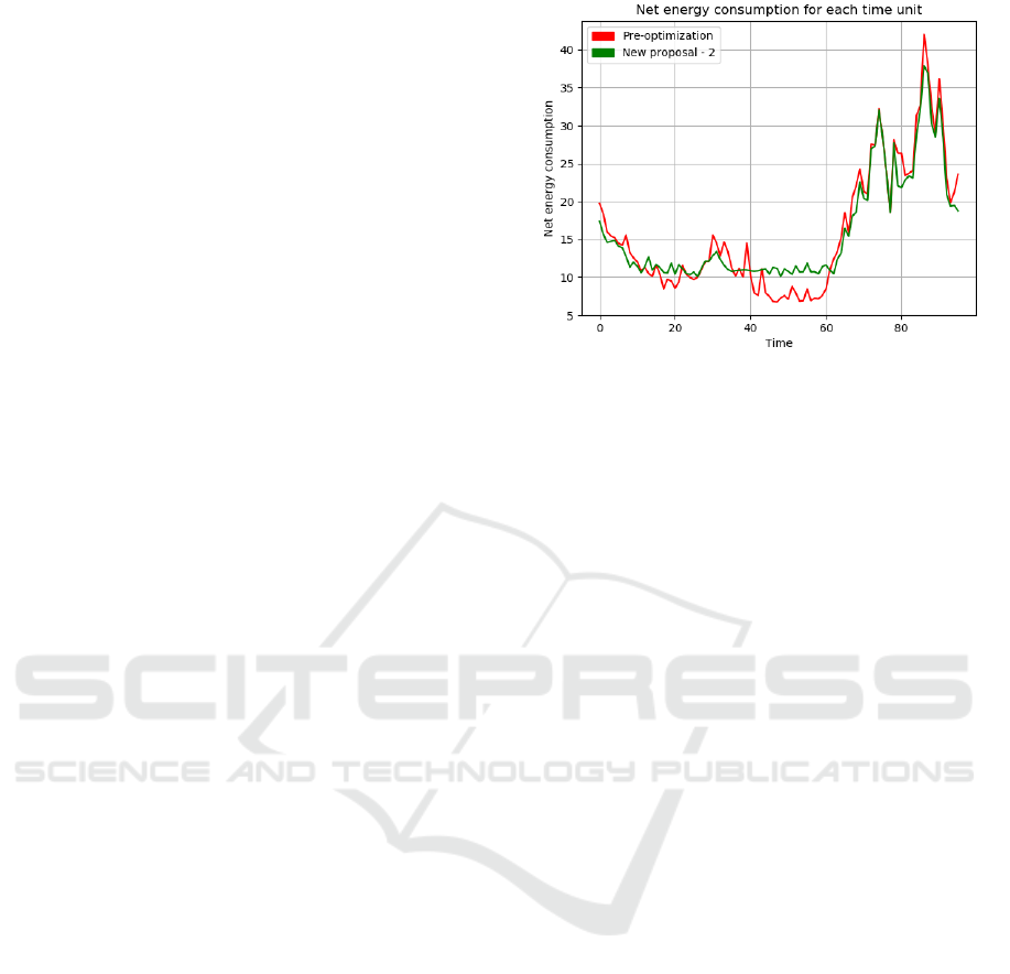
Finally, we report in graphical form the conse-
quences of the game to the daily net consumption
through the grid, which achieves an effect of peak-
shaving/valley-filling. We took as example the case
with 4 prosumers and 36 consumers, although all
cases present the same behavior. In Figure 1 the dif-
ference between production and consumption of en-
ergy is shown at each time unit, before and after opti-
mization.
6 CONCLUSIONS AND FUTURE
WORK
Local energy communities and peer-to-peer energy
trading are expected to be important components of
future energy system. This study investigated dif-
ferent mechanisms for regulating energy exchanges
between agents in local energy communities. The
agents are assumed to act in their own self-interest
when optimizing energy usage. The market mecha-
nisms are designed to incentivize production and self-
consumption of locally produced renewable energy
while matching supply and demand.
The proposed design exhibits advantageous the-
oretical properties when compared with some exist-
ing market mechanisms. The results obtained by sim-
ulations using real-world data reveal that incentives
Figure 1: Graph of net consumption of energy before and
after the optimization. The x axis indicates the time units
through the day, while on the y axis is indicated the differ-
ence between total consumption and production through the
grid. We have depicted the values before the optimization
(in red) and after the optimization (in green). It has to be
remarked that the shiftable loads were randomly allocated
through the day in the initial configuration.
offered by the proposed mechanisms in the form of
buying and selling prices lead more sustainable be-
haviours of energy communities. Consumers sched-
ule their consumption in periods with an intensive in-
jection of renewable energy whereas producers are
given a high reward that help discouraging them
from curtailment, which can appear under other ap-
proaches.
As future work we intend to investigate how the
proposed mechanisms behave when diverse sources
of flexibility are available including heating systems
and storage units.
ACKNOWLEDGEMENTS
This research has received funding from the European
Union’s Horizon 2020 research and innovation pro-
gram under grant agreement No 774431 (DRIvE).
REFERENCES
Capodieci, N., Pagani, G., Cabri, G., and Aiello, M.
(2011). Smart meter aware domestic energy trading
agents. In First International E-Energy Market
Challenge Workshop (co-located with ICAC’11).
ACM Press. Relation: https://www.rug.nl/fmns-
research/bernoulli/index Rights: University of
Groningen, Johann Bernoulli Institute for Mathemat-
ics and Computer Science.
Commission, T. E. (2013). European commission guidance
for the design of renewables support schemes, in: De-
ICAART 2020 - 12th International Conference on Agents and Artificial Intelligence
48

livering the internal market in electricity and making
the most of public intervention. Technical report, The
European Commission.
Ilic, D., da Silva, P. G., Karnouskos, S., and Griesemer,
M. (2012). An energy market for trading electricity
in smart grid neighbourhoods. In 6th IEEE Interna-
tional Conference on Digital Ecosystems and Tech-
nologies, DEST 2012, Campione d’Italia, Italy, June
18-20, 2012, pages 1–6.
Kok, J. K., Warmer, C. J., and Kamphuis, I. G. (2005).
Powermatcher: multiagent control in the electricity in-
frastructure. In 4rd International Joint Conference on
Autonomous Agents and Multiagent Systems (AAMAS
2005), July 25-29, 2005, Utrecht, The Netherlands -
Special Track for Industrial Applications, pages 75–
82.
Lilliu, F., Loi, A., Reforgiato Recupero, D., Sisinni, M.,
and Vinyals, M. (2019a). An uncertainty-aware op-
timization approach for flexible loads of smart grid
prosumers: A use case on the cardiff energy grid. Sus-
tainable Energy, Grids and Networks, 20:100272.
Lilliu, F., Vinyals, M., Denysiuk, R., and Reforgiato Recu-
pero, D. (2019b). A novel payment scheme for trad-
ing renewable energy in smartgrid. In Proceedings of
the Tenth International Conference on Future Energy
Systems, e-Energy 2019, Phoenix, United States, June
25-28, 2019, page To appear.
Loni, A. and Parand, F. (2017). A survey of game theory
approach in smart grid with emphasis on cooperative
games. In 2017 IEEE International Conference on
Smart Grid and Smart Cities (ICSGSC), pages 237–
242.
Mihaylov, M., Jurado, S., Avellana, N., Razo-Zapata, I. S.,
Moffaert, K. V., Arco, L., Bezunartea, M., Grau, I.,
Ca
˜
nadas, A., and Now
´
e, A. (2015). SCANERGY: a
scalable and modular system for energy trading be-
tween prosumers. In Proceedings of the 2015 Inter-
national Conference on Autonomous Agents and Mul-
tiagent Systems, AAMAS 2015, Istanbul, Turkey, May
4-8, 2015, pages 1917–1918.
Mihaylov, M., Jurado, S., Avellana, N., Van Moffaert, K.,
de Abril, I. M., and Now
´
e, A. (2014). Nrgcoin: Vir-
tual currency for trading of renewable energy in smart
grids. In European Energy Market (EEM), 2014 11th
International Conference on the, pages 1–6. IEEE.
Mihaylov, M., R
˘
adulescu, R., Razo-Zapata, I., Jurado, S.,
Arco, L., Avellana, N., and Now
´
e, A. (2019). Com-
paring stakeholder incentives across state-of-the-art
renewable support mechanisms. Renewable Energy,
131:689–699.
Nguyen, H. K., Song, J. B., and Han, Z. (2012). Demand
side management to reduce peak-to-average ratio us-
ing game theory in smart grid. In 2012 Proceed-
ings IEEE INFOCOM Workshops, Orlando, FL, USA,
March 25-30, 2012, pages 91–96.
Rad, A. H. M., Wong, V. W. S., Jatskevich, J., Schober, R.,
and Leon-Garcia, A. (2010). Autonomous demand-
side management based on game-theoretic energy
consumption scheduling for the future smart grid.
IEEE Trans. Smart Grid, 1(3):320–331.
Rosen, J. B. (1965). Existence and uniqueness of equilib-
rium points for concave n-person games. Economet-
rica, 33(3):520–534.
Saad, W., Han, Z., Poor, H. V., and Basar, T. (2012). Game-
theoretic methods for the smart grid: An overview
of microgrid systems, demand-side management, and
smart grid communications. IEEE Signal Process.
Mag., 29(5):86–105.
Sisinni, M., Sleiman, H., Vinyals, M., Oualmakran, Y.,
Pankow, Y., Grimaldi, I., Genesi, C., Espeche, J., Di-
bley, M., Yuce, B., Elshaafi, H., and McElveen, S.
(2016). D2.2 - mas
2
tering platform design document.
MAS
2
TERING public reports.
Soliman, H. M. and Leon-Garcia, A. (2014). Game-
theoretic demand-side management with storage de-
vices for the future smart grid. IEEE Trans. Smart
Grid, 5(3):1475–1485.
Peer-to-peer Energy Trading for Smart Energy Communities
49