Data-driven Algorithm for Scheduling with Total Tardiness

Michal Bou

ska

1,2 a

, Anton

ın Nov

1,2 b

, P

remysl

ucha

1 c

, Istv

an M

odos

1,2 d

and Zden

ek Hanz

alek

1 e

Czech Institute of Informatics, Robotics and Cybernetics, Czech Technical University in Prague,

Jugosl

avsk

ych partyz

u 1580/3, Prague, Czech Republic

Czech Technical University in Prague, Faculty of Electrical Engineering, Department of Control Engineering,

Karlovo n

est

ı 13, Prague, Czech Republic

Keywords:

Single Machine Scheduling, Total Tardiness, Data-driven Method, Deep Neural Networks.

Abstract:

In this paper, we investigate the use of deep learning for solving a classical N P -hard single machine schedul-

ing problem where the criterion is to minimize the total tardiness. Instead of designing an end-to-end machine

learning model, we utilize well known decomposition of the problem and we enhance it with a data-driven

approach. We have designed a regressor containing a deep neural network that learns and predicts the criterion

of a given set of jobs. The network acts as a polynomial-time estimator of the criterion that is used in a single-

pass scheduling algorithm based on Lawler's decomposition theorem. Essentially, the regressor guides the

algorithm to select the best position for each job. The experimental results show that our data-driven approach

can efﬁciently generalize information from the training phase to signiﬁcantly larger instances (up to 350 jobs)

where it achieves an optimality gap of about 0.5%, which is four times less than the gap of the state-of-the-art

NBR heuristic.

1 INTRODUCTION

The classical approaches for solving combinatorial

problems have several undesirable properties. First,

solving instances of an N P -Hard problem to op-

timality consumes an unfruitful amount of compu-

tational time. Second, there is no well-established

method how to utilize the solved instances for im-

proving the algorithm or recycling the solutions for

the unseen instances. Finally, the development of ef-

ﬁcient heuristic rules requires a substantial time de-

voted to the research. To address these issues, we

investigate the use of deep learning which is able to

derive knowledge from the already solved instances

of a classical scheduling N P -hard Single Machine

Total Tardiness Problem (SMTTP) and estimate the

optimal value of an unseen SMTTP instance. This is

the ﬁrst successful application of deep learning to the

scheduling problem; we successfully integrated the

deep neural network into a known decomposition al-

gorithm and outperformed the state-of-the-art heuris-

tics. With this, we are able to solve instances with

https://orcid.org/0000-0002-8034-2531

https://orcid.org/0000-0003-2203-4554

https://orcid.org/0000-0003-4895-157X

https://orcid.org/0000-0003-4692-1625

https://orcid.org/0000-0002-8135-1296

hundreds of jobs, which is signiﬁcantly more than,

e.g., an end-to-end approach (Vinyals et al., 2015)

that solves Traveling Salesman Problem with about

50 nodes. Our proposed approach outperforms the

state-of-the-art heuristic for SMTTP.

1.1 Problem Statement

The combinatorial problem studied in this paper is de-

noted as 1||

∑

in Graham’s notation of scheduling

problems (Graham et al., 1979). Let J = {1,..., n} be

a set of jobs that has to be processed on a single ma-

chine. The machine can process at most one job at a

time, the execution of the jobs cannot be interrupted,

and all the jobs are available for processing at time

zero. Each job j ∈ J has processing time p

∈ Z

≥0

and due date d

∈ Z

≥0

. Let π : {1,.. .,n} 7→ {1, ... ,n}

be a bijective function representing a sequence of the

jobs, i.e., π(k) ∈ J is the job at position k in sequence

π. For a given sequence π, tardiness of job π(k) is de-

ﬁned as T

π(k)

= max



∑

π(k

)



− d

π(k)



. The

goal of the scheduling problem is to ﬁnd a sequence

which minimizes the total tardiness, i.e.,

∑

j∈J

. The

problem is proven to be N P -hard (Du and Leung,

1990).

In the rest of the paper, we use the following two

deﬁnitions to describe the ordering of the jobs:

Bouška, M., Novák, A., Š˚ucha, P., Módos, I. and Hanzálek, Z.

Data-driven Algorithm for Scheduling with Total Tardiness.

DOI: 10.5220/0008915300590068

In Proceedings of the 9th International Conference on Operations Research and Enterprise Systems (ICORES 2020), pages 59-68

ISBN: 978-989-758-396-4; ISSN: 2184-4372

1. earliest due date (edd): if 1 ≤ j < j

≤ n then ei-

ther (i) d

< d

or (ii) d

= d

∧ p

≤ p

2. shortest processing time (spt): if 1 ≤ j < j

≤ n

then either (i) p

< p

or (ii) p

= p

∧ d

≤ d

1.2 Contribution and Outline

This paper addresses a single machine total tardiness

scheduling problem using a machine learning tech-

nique. Unlike some existing works, for example,

(Vinyals et al., 2015), we do not purely count on ma-

chine learning, but we combine it with the known ap-

proaches from OR domain. The advantage of our ap-

proach is that it can extract speciﬁc knowledge from

data, i.e., already solved instances, and use it to solve

the new ones. The experimental results show two

important observations. First, our algorithm outper-

forms the state-of-the-art heuristic (Holsenback and

Russell, 1992), and it also provides better results

on some instances than the exact state-of-the-art ap-

proach (Garraffa et al., 2018) with a time limit. Sec-

ond, the proposed algorithm is capable of generaliz-

ing the acquired knowledge to solve instances that

were not used in the training phase and also signiﬁ-

cantly differ from the training ones, e.g., in the num-

ber of jobs or the maximal processing time of jobs.

The rest of the paper is structured as follows.

In Section 2, we present a review of literature for

SMTTP and combination of operations research (OR)

and machine learning (ML). Section 3 describes our

approach integrating a regressor into the decomposi-

tion and analyzes it’s time complexity. We present

results for standard benchmark instances for SMTTP

in Section 4. Finally, the conclusion is drawn in Sec-

tion 5.

2 RELATED WORK

The ﬁrst part of the literature overview is based on

the extensive survey addressing SMTTP published by

(Koulamas, 2010) which we further extend with the

description of the current state-of-the-art algorithms.

The second part maps existing work in machine learn-

ing related to solving combinatorial problems.

2.1 SMTTP

In 1977 it was shown by Lawler (Lawler, 1977) that

the weighted single machine total tardiness problem

is N P -Hard. However, it took more than a decade to

prove that the unweighted variant of this problem is

N P -Hard as well (Du and Leung, 1990).

Lawler (Lawler, 1977) proposes a pseudo-

polynomial (in the sum of processing times) algo-

rithm for solving SMTTP. The algorithm is based

on a decomposition of the problem into subproblems.

The decomposition selects the job with the maximum

processing time and tries all the positions following

its original position in the edd order. For each po-

sition, two subproblems are generated; the ﬁrst sub-

problem contains all the jobs preceding the job with

the maximum processing time and the second sub-

problem contains all the jobs following the job with

the maximum processing time. In addition, Lawler

introduces rules for ﬁltering the possible positions of

the job with the maximum processing time. This al-

gorithm can solve instances with up to one hundred

jobs. F. Della Croce et al. (Della Croce et al., 1998)

proposed a spt decomposition which selects the job

with the minimal due date and tries all the positions

preceding its original position in spt order. Similarly

as with the Lawler’s decomposition, two subproblems

are generated where the ﬁrst subproblem contains all

the jobs preceding the job with the minimal due date

time and the second subproblem contains all the jobs

following the job with the minimal due date. F. Della

Croce et al. combined both edd decomposition and

spt decomposition together, this presented algorithm

is able to solve instances with up to 150 jobs. Finally,

Szwarc et al. (Szwarc et al., 1999) integrate the dou-

ble decomposition from (Della Croce et al., 1998) and

a split procedure from (Szwarc and Mukhopadhyay,

1996). This algorithm was the state-of-the-art method

for a long time with the ability to solve instance with

up to 500 jobs.

Recently, Garraffa et al. (Garraffa et al., 2018)

proposed Total Tardiness Branch-and-Reduce Algo-

rithm (TTBR), which infers information about nodes

of the search tree and merges nodes related to the

same subproblem. This is the fastest known exact al-

gorithm for SMTTP to this date and is able to solve

instances with up to 1300 jobs.

Exact algorithms, such as the ones mentioned

above, have very large computation times while the

optimal solution is rarely needed in practice. Hence,

heuristic algorithms are often more practical. Exist-

ing heuristics algorithm can be categorized into the

following three major groups.

The ﬁrst group of heuristics creates a job order

and schedule the jobs according this order, i.e., list

scheduling algorithms. There are various methods

for creating a job order. The easiest one is to sort

job by Earliest Due Date rule (edd). A more efﬁ-

cient algorithm called NBR was proposed in (Holsen-

back and Russell, 1992). NBR is a constructive lo-

cal search heuristic which starts with job set J sorted

ICORES 2020 - 9th International Conference on Operations Research and Enterprise Systems

by edd and constructs the schedule from the end by

exchanging two jobs. Panwalkar et al. (Panwalkar

et al., 1993) proposes constructive local search heuris-

tic PSK, which starts with job set J sorted by spt and

constructs the schedule from the start by exchang-

ing two jobs. Russel and Holsenback (Russell and

Holsenback, 1997) compares PSK and NBR heuris-

tic, and conducted that neither heuristic is inferior

to another one. However, NBR ﬁnds a better solu-

tions in more cases. The second group of heuris-

tics is based on Lawler decomposition rule (Lawler,

1977). In this case, heuristic evaluates each child of

the search tree node and the most promising child

is expanded. This heuristic approach is evaluated in

(Potts and Van Wassenhove, 1991) with edd heuris-

tic as a guide for the search. The third group of

heuristics are metaheuristics. (Potts and Van Wassen-

hove, 1991), (Antony and Koulamas, 1996), (Ben-

Daya and Al-Fawzan, 1996) present simulated an-

nealing algorithm for SMTTP. Genetic algorithms

applied to SMTTP are described in (Dimopoulos and

Zalzala, 1999), (S

uer et al., 2012), whereas (Bauer

et al., 1999), (Cheng et al., 2009) propose to use ant

colony optimization for this scheduling problem. All

the reported results in the previous studies are for in-

stance sizes up to 100 jobs. However, these instances

are solvable by the current state-of-the-art exact algo-

rithm in a fraction of second.

2.2 Machine Learning Integration to

Combinatorial Optimization

Problems

The integration of ML to combinatorial optimization

problems has several difﬁculties. As ﬁrst, ML models

are often designed with feature vectors having pre-

deﬁned ﬁxed size. On the other hand, instances of

scheduling problems are usually described by a vari-

able number of features, e.g., variable number of jobs.

This issue can be addressed by recurrent networks

and, more recently, by encoder-decoder type of ar-

chitectures. Vinyals (Vinyals et al., 2015) applied an

architecture called Pointer Network that, given a set

of graph nodes, outputs a solution as a permutation of

these nodes. The authors applied the Pointer Network

to Traveling Salesman Problem (TSP), however, this

approach for TSP is still not competitive with the best

classical solvers such as Concorde (Applegate et al.,

2006) that can ﬁnd optimal solutions to instances with

hundreds nodes in a fraction of second. Moreover, the

output from the Pointer Network needs to be corrected

by the beam-search procedure, which points out the

weaknesses of this end-to-end approach. Pointer Net-

work has achieved optimality gap around 1% for in-

stance with 20 nodes after performing beam-search.

Second difﬁculty with training a ML model is

with acquisition of training data. Obtaining one train-

ing instance usually requires solving a problem of

the same complexity like the original problem it-

self. This issue can be addressed with reinforcement

learning paradigm. Deudon et al. (Deudon et al.,

2018) used encoder-decoder architecture trained with

REINFORCE algorithm to solve 2D Euclidean TSP

with up to 100 nodes. It is shown that (i) repeti-

tive sampling from the network is needed, (ii) ap-

plying well-known 2-opt heuristic on the results still

improves the solution of the network, and (iii) both

the quality and runtime are worse than classical ex-

act solvers. Similar approach is described in (Kool

and Welling, 2018) which, if it is treated as a greedy

heuristic, beats weak baseline solutions (from the op-

erations research perspective) such as Nearest Neigh-

bor or Christoﬁdes algorithm on small instances. To

be competitive in terms of quality with more rele-

vant baselines such as Lin-Kernighan heuristics, they

perform multiple sampling from the model and out-

put the best solution. Moreover, they do not directly

compare their approach with state-of-the-art classi-

cal algorithms while admitting that off-the-shelf Inte-

ger Programming solver Gurobi solves optimally their

largest instances within 1.5 s.

Khalil et al. (Khalil et al., 2017) present an inter-

esting approach for learning greedy algorithms over

graph structures. The authors show that their S2V-

DQN model can obtain competitive results on MAX-

CUT and Minimum Vertex Cover problems. For TSP,

S2V-DQN performs about the same as 2-opt heuris-

tics. Unfortunately, the authors do not compare run-

times with Concorde solver.

Milan et al. (Milan et al., 2017) presents a

data-driven approximation of solvers for N P -hard

problems. They utilized a Long Short-Term Mem-

ory (Hochreiter and Schmidhuber, 1997) (LSTM) net-

work with a modiﬁed supervised setting. The reported

results on the Quadratic Assignment Problem show

that the network’s solutions are worse than general

purpose solver Gurobi while having the essentially

identical runtime.

Integration of ML with scheduling problems has

received a little attention so far. Earlier attempts of

integrating neural networks with job-shop scheduling

are (Zhou et al., 1991) and (Jain and Meeran, 1998).

However, their computational results are inferior to

the traditional algorithms, or they are not extensive

enough to assess their quality. An alternative use of

ML in scheduling domain is focused on the criterion

function of the optimization problems. For example,

authors in (V

aclav

ık et al., 2016) address a nurse ros-

Data-driven Algorithm for Scheduling with Total Tardiness

tering problem and improved the evaluation of the so-

lutions’ quality without calculating their exact crite-

rion values. They propose a classiﬁer, implemented

as a neural network, able to determine whether a cer-

tain change in a solution leads to a better solution or

not. This classiﬁer is then used in a local search al-

gorithm to ﬁlter out solutions having a low chance

to improve the criterion function. Nevertheless, this

approach is sensitive to changes in the problem size,

i.e., the size of the schedule of nurses. If the size is

changed, a new neural network must be trained. An-

other method, which does not directly predict a so-

lution to the given instance, is proposed in (V

aclav

ık

et al., 2018). In this case, an online ML technique is

integrated into an exact algorithm where it acts as a

heuristic. Speciﬁcally, the authors use regression for

predicting the upper bound of a pricing problem in a

Branch-and-Price algorithm. Correct prediction leads

to faster computation of the pricing problem while in-

correct prediction does not affect the optimality of the

algorithm. This method is not sensitive to the change

of the problem size; however, it is designed specif-

ically for the Branch-and-Price approach and cannot

be generalized to other approaches.

3 PROPOSED DECOMPOSITION

HEURISTIC ALGORITHM

In this section, we introduce Heuristic Optimizer

using Regression-based Decomposition Algorithm

(HORDA) for Single Machine Total Tardiness Problem

(SMTTP). This heuristic effectively combines the

well-know properties of SMTTP and the data-driven

approach. Moreover, this paper proposes a methodol-

ogy for designing data-driven heuristics for schedul-

ing problems where good estimator of the optimiza-

tion criterion can be obtained to guide the search.

This section is structured as follows. First of all,

we summarize decompositions used in the algorithm.

As the second, we describe HORDA. Next we con-

tinue by discussing the architecture of the regressor,

its integration into SMTTP decompositions, and de-

scribe the training of the neural network. Finally, we

analyze the time complexity of HORDA algorithm.

3.1 SMTTP Decompositions

Firstly, we describe two different decomposition ap-

proaches for SMTTP. The reason is that every state-

of-the-art exact algorithm for SMTTP is based on

these two decompositions.

First decomposition, introduced by Lawler

(Lawler, 1977), uses edd (earliest due date) order

in which it selects position for job j

p-max

, i.e., a

job with the maximal processing time from job set

J (in case of tie, j

p-max

is the job with the larger

index in edd order). Lawler proves that there

exists position k ∈ { j

p-max

,.. .,n} in the edd order

such that at least one optimal solution exists where

p-max

is preceded by all jobs {1,. .., k} \ { j

p-max

}

and followed by all jobs {k + 1,.. .,n}. Let us

denote set of positions { j

p-max

,.. .,n} as K

edd

. This

property leads to the following exact decomposition

algorithm. First, let P

edd

: P (J) × [1,.. .,n] → P (J)

and F

edd

: P (J) × [1, ... , n] → P (J) be functions

which for job set J and position k return subproblem

with jobs {1,... ,k} \ { j

p-max

} and {k + 1,. ..,n},

respectively. Where P (J) is powerset of J. Thus, for

each eligible position k ∈ { j

p-max

,.. .,n}, the problem

is decomposed into two subproblems deﬁned by

edd

(J, k) and F

edd

(J, k) such that jobs j

p-max

neither in P

edd

nor in F

edd

. Let Z (J) denote the

optimal criterion value for job set J computed as

Z (J) = min

k∈K

edd

Z (J,k) , (1)

where

Z (J,k) = Z



edd

(J, k)



max





0, p

− d

∑

j∈P

edd

(J,k)







edd

(J, k)



(2)

The optimal solution to the instance is found by recur-

sively selecting the position k with the minimal crite-

rion Z.

The second decomposition(Della Croce et al.,

1998) introduced by Della Croce et al. uses spt or-

der in which it selects position for job j

d-min

. We re-

fer to this decomposition as spt decomposition. Let

us deﬁne j

d-min

job as a job with the minimal due

date from job set J (in case of tie, j

d-min

is the job

with the smaller index in the spt order). Similarly

as in the edd decomposition proposed by Lawler,

Della Croce et al. (Della Croce et al., 1998) prove

that for job j

d-min

in spt order there exists position

k ∈ {1,.. ., j

d-min

} such that in at least one optimal so-

lution j

d-min

is preceded by job set generated by func-

tion P

spt

: P (J) × [1,.. .,n] → P (J). P

spt

(J, k) returns

job set with ﬁrst k jobs selected from {1,. .., j

d-min

}

which are then sorted by edd. Job j

d-min

is followed

by job set F

spt

: P (J) × [1, . .., n] → P (J) with all the

others jobs. The set of positions k ∈ {1, ... , j

d-min

} is

denoted as K

spt

. One may use the spt decomposition

in the same recursive way as edd decomposition to

ﬁnd the optimal solution.

ICORES 2020 - 9th International Conference on Operations Research and Enterprise Systems

The efﬁciency of both decomposition approaches

is signiﬁcantly inﬂuenced by the branching factor.

Here, the branching factor is equal to the number of

eligible positions where job j

p-max

∈ K

edd

( j

d-min

∈

spt

) can be placed. The number of eligible posi-

tions can be reduced by ﬁltering rules described in

(Lawler, 1977) and (Szwarc et al., 1999). Let us de-

note that

edd

, K

spt

are the sets K

edd

, K

spt

ﬁltered by

rules from (Szwarc et al., 1999) respectively.

3.2 HORDA

Even though algorithms using decompositions pro-

posed in (Lawler, 1977) and (Della Croce et al., 1998)

are very efﬁcient, their time complexity exponentially

grows with the number of jobs. Our HORDA algo-

rithm avoids this exponential growth by pruning the

search tree ruled by the polynomial-time estimation

of (2) produced by a neural network. The estimations

of Z (J,k) and Z (J) are denoted as

Z (J,k) and

Z (J),

respectively.

HORDA algorithm is outlined in Algorithm 1. To

increase the efﬁciency of the solution space search,

our HORDA algorithm combines the power of both de-

compositions (Lawler, 1977) and (Della Croce et al.,

1998) in the following way. The HORDA algorithm

generates (lines 5 and 6) two sets of eligible positions

edd

and K

spt

by either edd or spt decomposition

which are ﬁltered by state-of-the-art rules (Szwarc

and Mukhopadhyay, 1996). Then, the set with the

minimal cardinality is selected (lines 7 - 12) for the

recursive expansion; we refer to the selected set as K.

After obtaining positions set K, the algorithm

greedily selects k

∗

position having the minimal esti-

mation

Z (line 13). Next, the algorithm recursively

explores job sets P(J,k

∗

) and F (J, k

∗

), and result-

ing partial sequences are stored as vectors before and

after respectively (lines 14 and 15). Finally, the al-

gorithm merges {before, k

∗

,after} into one sequence,

which is returned as the resulting schedule (line 17).

Note that job sets with less or equal than 5 jobs are

solved to optimality by an exact solver (Total Tardi-

ness Branch-and-Reduce Algorithm (TTBR)) instead

of the decomposition.

3.3 Regressor

The proposed HORDA algorithm utilizes the regressor

estimation in the decomposition to guide the search

by selecting position k

∗

that minimizes the estimated

criterion

Z (see line 13). The quality of the estima-

tion signiﬁcantly affects the quality of the found solu-

tions. However, HORDA algorithm is not sensitive to

absolute error of the estimation, instead, it’s relative

Algorithm 1: Decomposition heuristic search

(HORDA).

Data: J

Result: HORDA ordered jobs

1 Function H O R D A (J):

2 if |J| ≤ 1 then

3 return toSequence(J)

4 end

/* Generate edd and spt positions

with respect to the filtering

rules */

5 K

edd

← genEDDPos(J)

6 K

spt

← genSPTPos(J)

7 if |K

edd

| ≤ |K

spt

| then

8 K ← K

edd

, P ← P

edd

, F ← F

edd

9 end

10 else

11 K ← K

spt

, P ← P

spt

, F ← F

spt

12 end

/* Where

Z is computed by

regressor. */

13 k

∗

← argmin

k∈K

(

Z (P(J,k)) + max(0, p

−

∑

j∈P(J,k)

) +

Z (F (J,k)))

14 before ← H O R D A (P(J, k

∗

))

15 after ← H O R D A (F (J,k

∗

))

/* join sequences into one */

16 order ← (before, k

∗

, after)

17 return order

error is important. Therefore, the proposed regres-

sor is based on neural networks that are known to be

successful for problems sensitive to relative error, for

example Google (Silver et al., 2016) applied them to

predict a policy in Monte Carlo Tree Search to solve

game of Go.

The architecture of our regressor using neural net-

work is illustrated in Figure 1. It has two main parts.

The ﬁrst one is the normalization of the input data, de-

scribed in Section 3.3.1. The second one is the neural

network, explained in Section 3.3.2.

3.3.1 Input Data Preprocessing

The speed of training and quality of the neural net-

work is affected by the preprocessing of the input in-

stances. There are two main reasons for the prepro-

cessing denoted as Norm in Figure 1. Firstly, prepro-

cessing of the input instance normalizes the instances,

and thus reduces the variability of input data denoted

X. For example, two neural network inputs differing

only in job order are, in fact, the same. Secondly, nu-

merical stability of the computation is improved by

Data-driven Algorithm for Scheduling with Total Tardiness

neural network

Norm

LSTM (512)

dense (1)

Norm

−1

Z(J) ∈ R

≥0

Figure 1: Regressor architecture.

the preprocessing. In our regression architecture, the

preprocessing has three main parts:

1. sorting of the input: we performed preliminary

experiments with various sorting options such as

edd, spt, reversed edd and reversed spt, among

which edd performed the best.

2. normalization of the input: the processing times

and due dates are divided by the sum of the pro-

cessing times in the instance.

3. appending additional features to the neural net-

work: each job has one additional feature which

is its position in X

X divided by the number of the

jobs.

The best practice in the neural network training

is to normalize value that is estimated by the neu-

ral network, denoted as y in Figure 1. In the train-

ing phase, the associated optimal criterion value of

each instance is divided by the sum of the process-

ing times. Alternatively, we evaluated one additional

criterion normalization Z/



n ·

∑

j∈J



. However, it

performed poorly. In the HORDA the estimation pro-

duced by the neural network has to be denormalized

by the inverse transformation (Norm

−1

in Figure 1) to

obtain the actual estimation of the total tardiness.

3.3.2 Neural Network

The input data for our neural network have several

similarities as the input data for nature language pro-

cessing (NLP) problems. Firstly, as well as NLP, our

data can be arbitraly large, i.e., the size of job set J is

unbounded; similarly, sentences in NLP can be arbi-

trarily long. In other research ﬁelds, such as computer

vision, this issue is mitigated by scaling the feature

vectors to a ﬁxed length. However, there is no sim-

ple and general way for scheduling problems how to

aggregate multiple jobs into one without losing nec-

essary information. Therefore, we use another tech-

nique of dealing with the varying length of the input

which are recurrent neural network (RNN) (Sunder-

meyer et al., 2012).

Our neural network for the criterion estimation

of J consists of two parts (the red box in Figure 1).

The ﬁrst layer is Long Short-Term Memory (Hochre-

iter and Schmidhuber, 1997) (LSTM), which receives

job set J as the input. The input X

X is a sequence of

features x

for every job j ∈ J. Each feature vector

consists of p

and d

with additional features de-

scribed below. The output of the last LSTM step is

passed into a dense layer which produces estimation

y of the criterion for X

3.4 Time Complexity of HORDA

In this section, we present the worst-case runtime of

HORDA. The most time consuming part of HORDA is

the estimation of

Z (J) by the regressor. The LSTM

layer produces

Z (J) in O(n) time and HORDA algo-

rithm evaluates the regressor 2 · n times to select posi-

tion k

∗

from K. Thus, the evaluation of all the estima-

tions for K takes O(n

). In the worst-case, when de-

composition repetitively removes one job, HORDA al-

gorithm makes O(n) selections of position k

∗

. There-

fore, the worst-case time complexity of HORDA al-

gorithm is O(n

). However, we note that the con-

stants present in the asymptotic complexit are fairly

low. Hence, it is efﬁcient in practice, as well.

4 EXPERIMENTAL RESULTS

In this section, we present the experimental results.

Firstly, we describe the training of the neural network,

also with the acquisition of a training dataset. Sec-

ondly, we describe the generation of the benchmark

instances. Then we compare our HORDA heuristic

with the state-of-the-art heuristic NBR (Holsenback

Table 1: Mean TTBR(Garraffa et al., 2018) runtimes

in seconds with respect to instance parameters for n ∈

{5,... , 500} and p

max

= 100. For parameters relative range

of due dates (rdd), and the average tardiness factor (tf ).

rdd/tf 0.2 0.4 0.6 0.8 1.0

0.2 0.07 2.16 5.16 1.64 0.04

0.4 0.04 0.36 1.64 0.05 0.04

0.6 0.04 0.06 0.47 0.04 0.04

0.8 0.04 0.04 0.07 0.04 0.04

1.0 0.04 0.04 0.04 0.04 0.04

ICORES 2020 - 9th International Conference on Operations Research and Enterprise Systems

Table 2: Optimality gap of HORDA, TTBR(Garraffa et al., 2018) and NBR(Holsenback and Russell, 1992) on instances with

max

= 100.

n TTBR NBR HORDA+NBR HORDA+NN

±25 time [s] gap [%] time [s] gap [%] time [s] gap [%] time [s]

225 1.05 ± 2.90 1.98 ± 0.58 0.06 ± 0.01 1.17 ± 0.47 1.19 ± 0.42 0.58 ± 0.30 5.03 ± 8.16

275 2.45 ± 4.19 2.12 ± 0.54 0.09 ± 0.02 1.31 ± 0.44 1.91 ± 0.62 0.57 ± 0.28 6.89 ± 9.62

325 4.72 ± 4.09 2.20 ± 0.50 0.12 ± 0.02 1.39 ± 0.43 2.87 ± 0.90 0.57 ± 0.37 9.25 ± 11.29

375 8.42 ± 4.75 2.27 ± 0.49 0.17 ± 0.03 1.46 ± 0.44 4.15 ± 1.31 1.23 ± 0.63 14.61 ± 13.52

425 14.42 ± 8.06 2.34 ± 0.46 0.21 ± 0.04 1.55 ± 0.41 5.52 ±1.71 1.71 ± 0.65 20.60 ± 17.00

Table 3: Optimality gap of heuristics on instances with p

max

= 5000.

n TTBR TTBR 10s NBR HORDA+NBR HORDA+NN

±25 time [s] gap [%] gap [%] gap [%] gap [%] time [s]

225 10.66 ± 9.20 0.17 ± 0.31 1.91 ± 0.60 1.10 ± 0.48 0.58 ± 0.27 3.58 ± 0.81

275 40.36 ± 32.24 0.77 ± 0.69 2.00± 0.54 1.20 ± 0.45 0.55 ±0.27 4.89 ± 1.02

325 92.30 ± 56.39 1.28 ± 0.86 2.27± 0.53 1.36 ± 0.47 0.53 ±0.33 6.61 ± 1.50

375 212.69 ± 122.14 1.87 ± 0.87 2.39 ± 0.47 1.50 ± 0.48 1.09 ± 0.60 10.32 ± 2.18

425 488.76 ± 265.88 2.64 ± 0.87 2.32 ± 0.44 1.52 ± 0.41 1.73 ± 0.64 14.96 ± 2.00

and Russell, 1992) and exact algorithm TTBR (Gar-

raffa et al., 2018). Finally, we discuss the advantages

of our proposed heuristic.

Experiments were run on a single-core of the

Xeon(R) Gold 6140 processor with a memory limit

set to 8GB of RAM. HORDA and NBR algorithms

were implemented in Python, and the neural network

is trained in Tensor Flow 1.14 on Nvidia GTX 1080

Ti. Source codes of TTBR algorithm were provided

by authors of (Garraffa et al., 2018) and it is imple-

mented in C.

4.1 Neural Network Training

We trained the neural network with Adam optimizer,

with learning rate set to 0.0001, early stop with pa-

tience equals to 5. Size of the LSTM layer is set to

512. For the neural network training, we generated

instances by scheme introduced by Potts and Wassen-

hove (Potts and Wassenhove, 1982). The scheme uses

two parameters; relative range of due dates (rdd),

and the average tardiness factor (tf ). The values of

rdd, tf typically used in the literature are rdd,tf ∈

{0.2,0.4,0.6, 0.8,1}. For each such rdd, tf and n ∈

{5,.. .,250}, we generated 5000 instances. There-

fore, the whole training dataset consists of 30625000

instances in total. Since we use a supervised learning

to train the neural network, we need optimal criterion

values that acts as labels.

It is easy to see that the dataset is enormous,

and it is necessary to solve millions of SMTTP in-

stances. However, this is not an issue since a sub-

stantial amount of the instances can be solved within

a fraction of a second. Moreover, the dataset can be

cheaply generated in the cloud, e.g., on the Amazon

EC2 cloud, the cost of generating the dataset is around

800$ and takes only ten days, which is signiﬁcantly

cheaper compared to the cost of a human expert de-

veloping a heuristic algorithm.

Furthermore, it is important to stress that our neu-

ral network is able to generalize to larger instance

than used in the training. Therefore, it is possible

to train the neural network on smaller instances and

solve larger ones both in terms of the number of jobs

and their parameters.

4.2 Benchmark Instances

Benchmark instances used in this paper were gen-

erated in the manner suggested by Potts and Van

Wassenhove in (Potts and Van Wassenhove, 1991)

and used in Section 4.1. Potts and Van Wassenhove

generate processing times of jobs uniformly on the

interval from 1 to 100. We deﬁne maximal process-

ing time p

max

and generate processing time of jobs

in instance uniformly on the interval from 1 to p

max

For p

max

= 100 and n ∈ {5,. .., 500}, we generated

25 sets of benchmarks differing in rdd and tf . Then

those instances were solved by TTBR algorithm. Ta-

ble 1 shows average runtimes in seconds over (rdd,tf )

∈ {0.2,0.4,0.6,0.8, 1}

. The results imply, that the

hardest instances occur for rdd = 0.2 and tf = 0.6

(highlighted in Table 1 in bold), therefore our experi-

ments concentrate on them. Nevertheless, it is impor-

tant to stress that the neural network is trained on the

whole range of values (rdd,tf ). First, we do not want

Data-driven Algorithm for Scheduling with Total Tardiness

200

250

300

350

400

450

NN Generalization

optimality gap [%]

NBR

HORDA+NBR

HORDA+NN

TTBR 10s

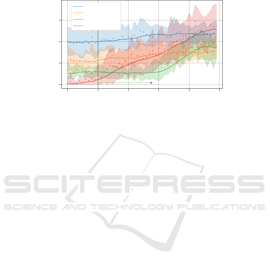
Figure 2: Optimality gap on instances with p

max

= 5000.

the algorithm to be limited to a speciﬁc class of in-

stances. Second, since our algorithm uses the decom-

positions, as described in Section 3.1, there is no guar-

antee that the subproblems have the same (rdd,tf ) pa-

rameterization as the input instance. In fact, during

the run of HORDA, the values of (rdd,tf ) in newly

emerged subproblems shift from the original ones.

4.3 Comparison with Existing

Approaches

In the ﬁrst experiment, summarized in Table 2, we

concentrate on the comparison with NBR heuristic.

The benchmark instances used in this experiment

were generated with p

max

= 100. Each row in the ta-

ble represents a set of 200 instances of size from range

[n−25,n+25). The optimal solution was obtained by

TTBR algorithm. The table compares NBR heuristic

with HORDA algorithm where the regressor is substi-

tuted by NBR heuristic (denoted HORDA+NBR), and

HORDA heuristic with the neural network regressor

(denoted HORDA+NN). These three approaches are

compared in terms of the average CPU time, and the

average quality of solutions, measured by the optimal-

ity gap in percent. All values are reported together

with their standard deviation.

Results are shown from n = 200. For smaller n

than 200, TTBR is able to ﬁnd the optimal solution un-

der a second, and because of this, the results of heuris-

tics are not relevant. The bold values in the table in-

dicate the best result over all the heuristic approaches

for the particular set of instances. The results show

that HORDA+NN has the best performance in terms of

the average optimality gap. In the case of the last data

set, the second heuristic HORDA+NBR is slightly bet-

ter. The reason is that the neural network was trained

only on instances with n ≤ 250. Therefore, one can

see that our neural network, used in the regressor, is

able to generalize the gained knowledge to instances

with n ≤ 400. On instances with n ≤ 325, the average

optimality gap of HORDA+NN is about 0.5%, which

outperforms all other methods. At the same time, we

have to admit that the heuristic is slower than TTBR

algorithm. Nevertheless, this is true only on instances

generated with p

max

= 100. On larger maximum pro-

cessing time, the CPU time of TTBR is signiﬁcantly

larger as will be seen in the next experiment.

In literature, benchmark instances for SMTTP are

usually generated with p

max

= 100, as it was used in

the previous experiment. Since SMTTP is applica-

ble in production and grid computing and p

max

can be

much longer in these ﬁelds, we introduce the follow-

ing experiments with maximal processing time p

max

equal to 5000. Table 3 compares our HORDA +NN and

HORDA+NBR heuristics with NBR, TTBR and TTBR

with runtime limited to 10 s denoted as TTBR10s. For

TTBR 10s, a 10 s limit is selected with respect to the

HORDA+NN algorithm runtime, since the runtime of

HORDA+NN on instances with up to n = 350 is un-

der 10 s. Please note that the identical regressor as in

Table 2 was used, i.e., the regressor was trained only

on instances with p

max

= 100. Hence, it demonstrates

neural network’s ability of generalization outside the

training processing time range.

One can observe from Table 2 and Table 3 that

the CPU time of HORDA +NN is almost the same for

both types of instances. However, this is not true for

TTBR where the CPU time is almost 30 times higher

for n = 425. Also, the CPU time of TTBR is more than

30 times higher for n = 425 and p

max

= 5000 com-

pared to HORDA+NN. If the runtime of TTBR is lim-

ited to 10 s, then HORDA +NN outperforms TTBR10s

ICORES 2020 - 9th International Conference on Operations Research and Enterprise Systems

on larger instances. Moreover, the optimality gap of

HORDA+NN is practically the same as in the previous

experiment with p

max

= 100.

The same experiment is shown in the form of a

graph in Figure 2. It compares the optimality gap

of NBR, TTBR with a time limit, HORDA +NBR, and

HORDA+NN. The bold lines in the graph represent

the moving average (last 5 samples) of optimality

gap of each method, and the colored areas represent

their standard deviation. HORDA +NN outperforms

HORDA+NBR about two times up to instances of size

n = 360. For instances with n ≥ 405, HORDA+NBR,

is slightly better. In addition, HORDA+NN also

outperforms TTBR 10s from n = 265. Furthermore,

HORDA+NN holds the average optimality gap around

0.5% for instances with up to 350 jobs. The same can

be observed on instances with p

max

= 100 (see Ta-

ble 2). Finally, the runtime of TTBR grows exponen-

tially with the growing size of the instance, in contrast

to polynomial runtime of HORDA+NN.

Concerning the heuristic using the neural network

(HORDA+NN), it is important to stress that for in-

stances with n > 250 the network has to generalize

the acquired knowledge since it was trained only on

instances with n ≤ 250. This fact is indicated in Fig-

ure 2 by a green vertical line. It can be seen that

HORDA+NN is able to generalize results to instances

having 100 more jobs than instances encountered in

the training phase with 50 times larger maximal pro-

cessing time (instances for the training phase were

generated with p

max

= 100).

5 CONCLUSION

To the best of our knowledge, this is the ﬁrst paper

addressing a scheduling problem using deep learn-

ing. Unlike the solution used in (Vinyals et al.,

2015), which tackled the Traveling Salesman Prob-

lem, we combined a state-of-the-art operations re-

search method with a DNN. The experimental results

show that our approach provides near-optimal solu-

tions very quickly and is also able to generalize the

acquired knowledge to larger instances without sig-

niﬁcantly affecting the quality of the solutions. Our

approach outperforms state-of-the-art heuristic NBR.

Our approach is shown to be competitive and in some

cases, superior to the previous state-of-the-art algo-

rithms. Hence, we believe that the proposed method-

ology opens new possibilities for the design of efﬁ-

cient heuristics algorithms.

ACKNOWLEDGEMENTS

The authors want to thank Vincent T’Kindt from

Universit de Tours for providing the source

code of TTBR algorithm. This work was sup-

ported by the European Regional Development

Fund under the project AI&Reasoning (reg. no.

CZ.02.1.01/0.0/0.0/15 003/0000466).

This work was supported by the Grant Agency of

the Czech Technical University in Prague, grant No.

SGS19/175/OHK3/3T/13.

REFERENCES

Antony, S. R. and Koulamas, C. (1996). Simulated anneal-

ing applied to the total tardiness problem. Control and

Cybernetics, 25:121–130.

Applegate, D., Bixby, R., Chvatal, V., and Cook, W. (2006).

Concorde TSP solver.

Bauer, A., Bullnheimer, B., Hartl, R. F., and Strauss,

C. (1999). An ant colony optimization approach

for the single machine total tardiness problem. In

Proceedings of the 1999 Congress on Evolution-

ary Computation-CEC99 (Cat. No. 99TH8406), vol-

ume 2, pages 1445–1450. IEEE.

Ben-Daya, M. and Al-Fawzan, M. (1996). A simulated

annealing approach for the one-machine mean tardi-

ness scheduling problem. European Journal of Oper-

ational Research, 93(1):61–67.

Cheng, T. E., Lazarev, A. A., and Gafarov, E. R. (2009).

A hybrid algorithm for the single-machine total tar-

diness problem. Computers & Operations Research,

36(2):308–315.

Della Croce, F., Tadei, R., Baracco, P., and Grosso, A.

(1998). A new decomposition approach for the single

machine total tardiness scheduling problem. Journal

of the Operational Research Society, 49(10):1101–

1106.

Deudon, M., Cournut, P., Lacoste, A., Adulyasak, Y., and

Rousseau, L.-M. (2018). Learning heuristics for the

tsp by policy gradient. In International Conference

on the Integration of Constraint Programming, Ar-

tiﬁcial Intelligence, and Operations Research, pages

170–181. Springer.

Dimopoulos, C. and Zalzala, A. (1999). A genetic

programming heuristic for the one-machine total

tardiness problem. In Proceedings of the 1999

Congress on Evolutionary Computation-CEC99 (Cat.

No. 99TH8406), volume 3, pages 2207–2214. IEEE.

Du, J. and Leung, J. Y. T. (1990). Minimizing total tardi-

ness on one machine is NP-Hard. Math. Oper. Res.,

15(3):483–495.

Garraffa, M., Shang, L., Della Croce, F., and T’Kindt, V.

(2018). An exact exponential branch-and-merge algo-

rithm for the single machine total tardiness problem.

Theoretical Computer Science, 745:133–149.

Data-driven Algorithm for Scheduling with Total Tardiness

Graham, R. L., Lawler, E. L., Lenstra, J. K., and Kan, A. R.

(1979). Optimization and approximation in determin-

istic sequencing and scheduling: a survey. Annals of

discrete mathematics, 5:287–326.

Hochreiter, S. and Schmidhuber, J. (1997). Long short-term

memory. Neural Comput., 9(8):1735–1780.

Holsenback, J. E. and Russell, R. M. (1992). A heuristic

algorithm for sequencing on one machine to minimize

total tardiness. Journal of the Operational Research

Society, 43(1):53–62.

Jain, A. S. and Meeran, S. (1998). Job-shop scheduling

using neural networks. International Journal of Pro-

duction Research, 36(5):1249–1272.

Khalil, E., Dai, H., Zhang, Y., Dilkina, B., and Song, L.

(2017). Learning combinatorial optimization algo-

rithms over graphs. In Advances in Neural Informa-

tion Processing Systems, pages 6348–6358.

Kool, W. and Welling, M. (2018). Attention solves your

TSP. arXiv preprint arXiv:1803.08475.

Koulamas, C. (2010). The single-machine total tardiness

scheduling problem: Review and extensions. Euro-

pean Journal of Operational Research, 202(1):1 – 7.

Lawler, E. L. (1977). A pseudopolynomial algorithm for se-

quencing jobs to minimize total tardiness. In Hammer,

P., Johnson, E., Korte, B., and Nemhauser, G., editors,

Studies in Integer Programming, volume 1 of Annals

of Discrete Mathematics, pages 331 – 342. Elsevier.

Milan, A., Rezatoﬁghi, S. H., Garg, R., Dick, A. R., and

Reid, I. D. (2017). Data-driven approximations to NP-

hard problems. In AAAI, pages 1453–1459.

Panwalkar, S., Smith, M., and Koulamas, C. (1993).

A heuristic for the single machine tardiness prob-

lem. European Journal of Operational Research,

70(3):304–310.

Potts, C. and Van Wassenhove, L. N. (1991). Single ma-

chine tardiness sequencing heuristics. IIE transac-

tions, 23(4):346–354.

Potts, C. and Wassenhove, L. V. (1982). A decomposition

algorithm for the single machine total tardiness prob-

lem. Operations Research Letters, 1(5):177 – 181.

Russell, R. and Holsenback, J. (1997). Evaluation of

greedy, myopic and less-greedy heuristics for the sin-

gle machine, total tardiness problem. Journal of the

Operational Research Society, 48(6):640–646.

Silver, D., Huang, A., Maddison, C. J., Guez, A., Sifre, L.,

Van Den Driessche, G., Schrittwieser, J., Antonoglou,

I., Panneershelvam, V., Lanctot, M., et al. (2016).

Mastering the game of go with deep neural networks

and tree search. nature, 529(7587):484.

uer, G. A., Yang, X., Alhawari, O. I., Santos, J., and

Vazquez, R. (2012). A genetic algorithm approach for

minimizing total tardiness in single machine schedul-

ing. International Journal of Industrial Engineering

and Management (IJIEM), 3(3):163–171.

Sundermeyer, M., Schl

uter, R., and Ney, H. (2012). Lstm

neural networks for language modeling. In Thirteenth

annual conference of the international speech commu-

nication association.

Szwarc, W., Della Croce, F., and Grosso, A. (1999). So-

lution of the single machine total tardiness problem.

Journal of Scheduling, 2(2):55–71.

Szwarc, W. and Mukhopadhyay, S. K. (1996). Decompo-

sition of the single machine total tardiness problem.

Operations Research Letters, 19(5):243–250.

aclav

ık, R., Novak, A.,

ucha, P., and Hanz

alek, Z.

(2018). Accelerating the branch-and-price algorithm

using machine learning. European Journal of Opera-

tional Research, 271(3):1055 – 1069.

aclav

ık, R.,

ucha, P., and Hanz

alek, Z. (2016). Roster

evaluation based on classiﬁers for the nurse rostering

problem. Journal of Heuristics, 22(5):667–697.

Vinyals, O., Fortunato, M., and Jaitly, N. (2015). Pointer

networks. In Advances in Neural Information Pro-

cessing Systems, pages 2692–2700.

Zhou, D. N., Cherkassky, V., Baldwin, T. R., and Olson,

D. E. (1991). A neural network approach to job-shop

scheduling. IEEE Transactions on Neural Networks,

2(1):175–179.

ICORES 2020 - 9th International Conference on Operations Research and Enterprise Systems