Semisupervised Classification of Anomalies Signatures
in Electrical Wafer Sorting (EWS) Maps
Luigi C. Viagrande
1,2 a
, Filippo L. M. Milotta
1,2 b
, Paola Giuffr
`
e
1
,
Giuseppe Bruno
1
, Daniele Vinciguerra
1
and Giovanni Gallo
2 c
1
STMicroelectronics, Catania, Italy
2
University of Catania, Catania, Italy
Keywords:
Semiconductor Manufacturing, Electrical Wafer Sorting Map, Wafer Map Clustering, Anomalies Signature
Classification, Yield Analysis.
Abstract:
We focused onto a very specific kind of data from semiconductor manufacturing called Electrical Wafer Sort-
ing (EWS) maps, that are generated during the wafer testing phase performed in semiconductor device fabri-
cation. Yield detractors are identified by specific and characteristic anomalies signatures. Unfortunately, new
anomalies signatures may appear among the huge amount of EWS maps generated per day. Hence, it’s unfea-
sible to define just a finite set of possible signatures, as this will not represent a real use-case scenario. Our goal
is anomalies signatures classification. For this purpose, we present a semisupervised approach by combining
hierarchical clustering to create the starting Knowledge Base, and a supervised classifier trained leveraging
clustering phase. Our dataset is daily increased, and the classifier is dynamically updated considering possible
new created clusters. Training a Convolutional Neural Network, we reached performance comparable with
other state-of-the-art techniques, even if our method does not rely on any labeled dataset and can be daily
updated. Our dataset is skewed and the proposed method was proved to be rotation invariant. The proposed
method can grant benefits like reduction of wafer test results review time, or improvement of processes, yield,
quality, and reliability of production using the information obtained during clustering process.
1 INTRODUCTION
Semiconductor manufacturing requires complex
equipment where each machine contains hundreds
of components, and thousands of failure points at
minimum. Yield across the entire line usually must
be very high, and there must be a continuous learning
process to keep in place the yield at high levels. New
products must be quickly brought up to high yield, as
the profit margins of these new products are often a
major source of profit in the semiconductor industry,
due to the high competitive environment. Given the
huge amount of data collected from each facility in
the industry, we fall within the context of Big Data.
This requires a proper data analysis and management,
that can bring to useful insights for increasing yield
rate or detect anomalies at early stages.
In this paper, we focus onto a very specific kind
a
https://orcid.org/0000-0003-2843-679X
b
https://orcid.org/0000-0002-9459-9530
c
https://orcid.org/0000-0002-6701-0620
of data called Electrical Wafer Sorting (EWS) maps.
These images are generated during the wafer testing
phase performed in semiconductor device fabrication.
A wafer is a round-shaped support containing several
“dies”. After testing, good dies are cut out from the
wafer and sent to the package phase. Instead, bad
ones were litterally “inked” to be easily recognized
and discarded when dies are extracted from the wafer.
Today, defective dies are not inked anymore, as this
can be done digitally, employing maps that can be
used for masking good and bad portions of the wafer.
Maps represent dies on the wafer and, accordingly to
a statistical binning approach, they can have several
values (i.e., good or failed during test stage 1, stage
2, and so on). For simplicity, we assume to handle
binary EWS maps, where white pixels identify failed
dies, while black pixels the good ones. Since many
yield detractors can impact production at the same
time, device engineers have to spend a lot of time ana-
lyzing EWS data to identify every yield detractor and
relative affected wafers before proceeding to in-depth
278
Viagrande, L., Milotta, F., Giuffrè, P., Bruno, G., Vinciguerra, D. and Gallo, G.
Semisupervised Classification of Anomalies Signatures in Electrical Wafer Sorting (EWS) Maps.
DOI: 10.5220/0008914402780285
In Proceedings of the 15th International Joint Conference on Computer Vision, Imaging and Computer Graphics Theory and Applications (VISIGRAPP 2020) - Volume 5: VISAPP, pages
278-285
ISBN: 978-989-758-402-2; ISSN: 2184-4321
Copyright
c
 2022 by SCITEPRESS – Science and Technology Publications, Lda. All rights reserved

(a) (b) (c) (d)
Figure 1: EWS maps showing the following characteristic
anomalies signatures: (a) Scratch, (b) Ring, (c) Spot, and
(d) Wheel. White pixels identify defective dies.
analysis and data mining to identify root causes. Usu-
ally, yield detractors can be identified by specific and
characteristic patterns, named EWS map signatures
(i.e., scratch, ring, spot, or wheel, as shown in Fig-
ure 1). These patterns are useful for investigating the
root causes that could be, for instance, related to an
equipment component failure, a drifting process, or
an integration of processes (May and Spanos, 2006).
Unfortunately, new anomalies signatures may appear
among the huge amount of EWS maps generated per
day (i.e., we are facing an open set problem). Hence,
it’s unfeasible to define just a finite set of possible sig-
natures, as this will not represent a real use-case sce-
nario. The automatic labeling of old and new anoma-
lies represents an interesting research issue with rele-
vant industrial applications.
Clearly, we are within the scope of unsupervised
learning, and we need to apply a clustering strategy.
Since the concept of cluster in data analysis has been
introduced, it has spanned through a wide range of
disciplines (Tvaronaviciene et al., 2015; Han et al.,
2001). Many real world problems, indeed, found
their solution on cluster analysis. In this paper, the
“objects” to cluster are real EWS maps acquired by
STMicroelectronics. We wish to aggregate the EWS
maps accordingly to their anomalies signatures. In
practical clustering applications, it is not known in
advance how many clusters have to be treated, and
their number may also change when different days of
production are considered. Although in certain cases
the number of clusters is already known, this does
not apply in our case, as said before. Many studies
have been carried out to estimate the optimal num-
ber of clusters for a given clustering task, but this
field is very challenging and existing methods still
have drawbacks (Wang et al., 2018). In our appli-
cation, the number of clusters is daily increased upon
dynamically data analysis. In the proposed method,
we have looked into the field of aggregative cluster-
ing, one of the earliest and most widely used cluster-
ing strategy (Balcan et al., 2014; Bryant and Berry,
2001). We have evidence of aggregative clustering
since 1950 (Ackermann et al., 2014).
Once clustering phase is completed, we will have
a dataset of EWS maps where each image will be as-
signed to a specific and unique cluster. Then, as in
a supervised approach, we may leverage the outcome
of clustering phase considering the assigned cluster-
ID as label for training a classifier. Indeed, this hybrid
approach is defined semisupervised learning, and it is
particularly meaningful as the manual classification
could lead to different results among different opera-
tors, who are biased by subjective interpretation of the
anomalies signatures. Clustering analysis was lever-
aged for anomalies signatures classification in recent
works (Zhang et al., 2013; Wu et al., 2014; Saqlain
et al., 2019; Jin et al., 2019). However, all of these
works applied supervised learning assuming a finite
set of just 9 anomalies signatures. They employed the
WM-811K dataset (WM-811K, 2018), that is made
of 811,457 wafer maps collected real-world fabrica-
tion. Images in the WM-811K dataset are similar to
EWS maps we employed in this work: in the for-
mer case images are labeled, while in the latter they
are not. One of the most recent related works on
anomalies signatures retrieval was focused onto wafer
defect maps (WDM) classification (Di Bella et al.,
2019). Even if WDM images look really similar to
EWS maps, we remark that defectivity analysis is a
test phase performed some steps before the EWS one.
Differently from the present work, a labeled dataset
with a set of finite classes was employed for WDM
classification, too.
In sum the contributions of this work are:
• Semisupervised Classifier: a new semisuper-
vised approach for classifying anomalies signa-
tures in EWS maps is presented, by combining an
unsupervised approach using a Hierarchical clus-
tering algorithm to create the starting Knowledge
base, and a supervised one through a classifier
trained leveraging clustering phase (Figure 2);
• Daily Update: our dataset can be daily increased,
and the classifier is dynamically updated consid-
ering possible new created clusters. The workflow
of our solution can be resumed in: daily arrival of
EWS maps, clustering of newcomer images into
previously created clusters, possible creation of
new clusters, anomalies signatures classification;
• Variable Number of Anomalies Signatures: we
are not considering a fixed number of anomalies
signatures, and the leveraged dataset does not con-
tain any label. This represents the typical scenario
of real use-case industrial applications.
The goal of this work is to create a tool to make as
automatic as possible the recognition of wafer anoma-
lies signatures. This is meaningful as upon classifica-
tion the industrial system can be able to automatically
Semisupervised Classification of Anomalies Signatures in Electrical Wafer Sorting (EWS) Maps
279

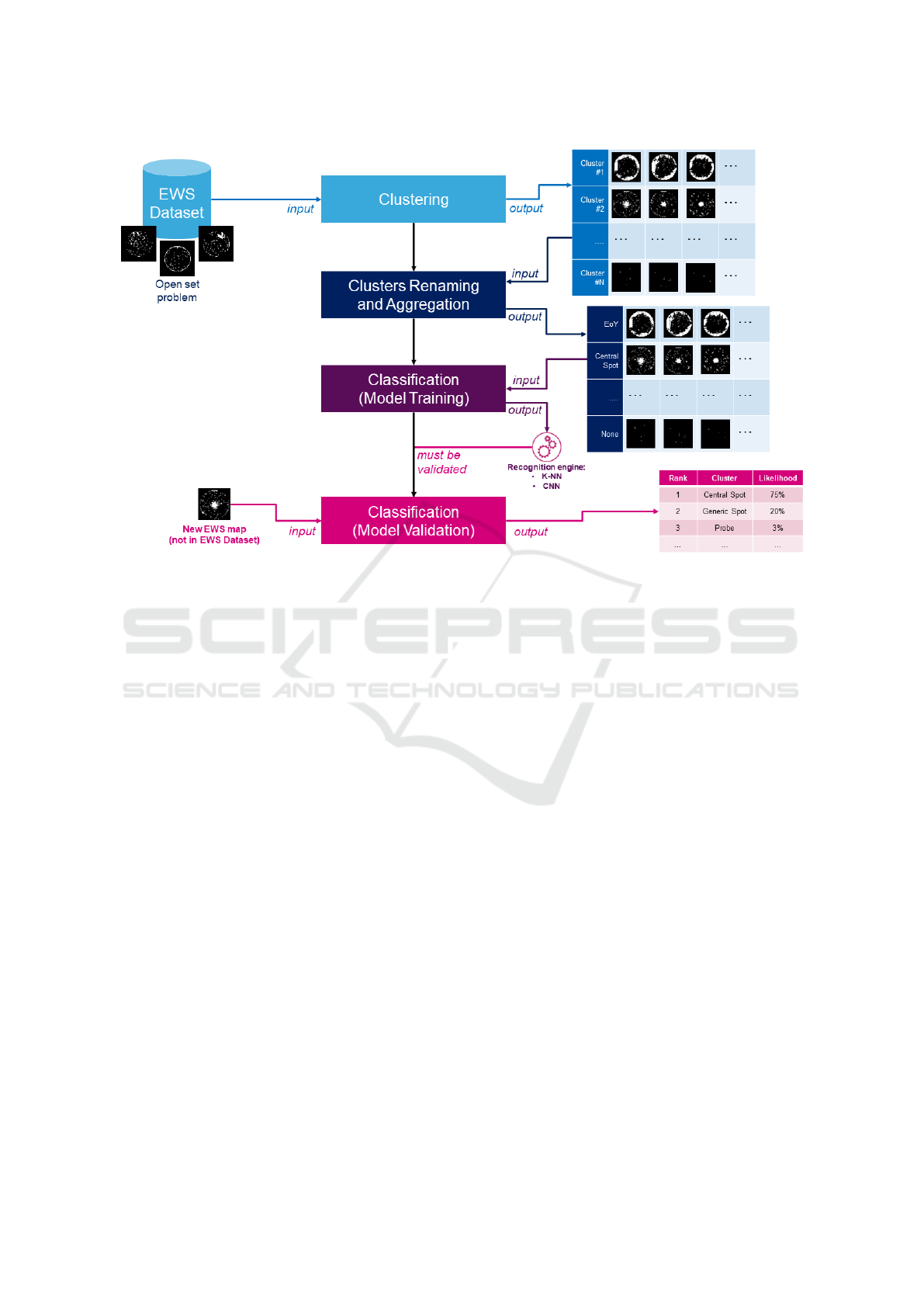
Figure 2: Overview workflow of the proposed approach.
choose (or at least suggest) either to discard a wafer or
to ship it to customer. The proposed method can also
grant benefits like reduction of wafer test results re-
view time, or improvement of processes, yield, qual-
ity, and reliability of production using the information
obtained during clustering process.
The remainder of the paper is organized as fol-
lows. In Section 2 we define our semisupervised
approach for anomalies signatures classification, de-
scribing in detail the clustering and classification
phases. Some cues about image descriptors, knowl-
edge base (i.e., the number of clusters), daily update,
and data augmentation, are given within this Section.
Then, in Section 3, we report our experimental re-
sults, showing clustering visual assessment, rotation
invariance of the proposed method, and performance
of both clustering and classification phases. Finally,
we conclude the paper with a final discussion and
some remarks for possible future works.
2 DATA AND METHODS
The proposed method is based onto a semisupervised
approach (Figure 2), that can be divided in two main
parts: the clustering and the classification phases (i.e.,
unsupervised and supervised learning). They are de-
scribed in order. Dataset was gradually incremented
during the several reported phases, so the dataset defi-
nition will be given together with the method descrip-
tion.
2.1 Clustering
In the clustering phase we firstly defined the descrip-
tors computed from EWS maps. Then, we described a
preliminary clustering phase, in which we assess the
cluster algorithm to be used in our experiments. In
this Section, we also defined the initial dataset and
the error measure for determining the number of clus-
ters. Finally, we introduced our knowledge base of
anomalies signatures.
2.1.1 Descriptors
There are several descriptors for labeled wafer maps
images (Wu et al., 2014). However, given the unla-
beled characteristic of our dataset, we decided to in-
vestigate two more general effective descriptors: Lo-
cal Binary Pattern (LBP) and Principal Components
(PC).
Local Binary Pattern (LBP): the LBP operator is
defined as a grey scale invariant texture operator. It
has become a popular approach in applications, in-
cluding visual inspection, and image analysis. Given
a grayscale image, the operator compares the 3×3
VISAPP 2020 - 15th International Conference on Computer Vision Theory and Applications
280

neighborhood of each pixel with this central pixel
value, and transforms the result to a binary number.
Then, image is represented through the histogram of
these computed binary numbers (Hadid et al., 2008).
Principal Components (PCs): the PCs are com-
puted through the Principal Component Analysis
(PCA). The PCA is an orthogonal linear transforma-
tion that modifies the data to a new coordinate sys-
tem in such a way to highlight their similarities and
differences (Mishra et al., 2017). Images with a res-
olution of 61×61 pixels are “vectorized”, that is they
are reshaped into a vector of 3,721 pixels (Turk and
Pentland, 1991). We decided to keep as many PCs
as needed to have at least the 80% of variance retain.
Typically, only 15 to 20 PCs survive over the 3,721
original ones. These PCs are used as descriptor for
the clustering phase.
2.1.2 Preliminary Clustering Phase
During the preliminary clustering phase, we collected
a first dataset of 296 images, with a resolution of
61×61 pixels. This tiny dataset was the only one
to be manually labeled by a team of experts, in or-
der to validate the preliminary clustering outcomes.
Among the many available clustering techniques, we
focused onto K-means, divisive hierarchical cluster-
ing and, particularly, on the aggregative hierarchical
clustering algorithm. We clustered the 296 images in
5 clusters. Then, clustering outcomes were validated
by experts. Indeed, the main purpose of this phase
was to select the clustering algorithm, and we chose
the aggregative hierarchical clustering.
Hierarchical clustering is an unsupervised algo-
rithm that subdivides the dataset in partitions lever-
aging a distance function. It produces a hierarchical
representation, with the lowest level of the hierarchy
counting n clusters, where n is the total number of ob-
servations. Instead, at the top level we have a single
cluster containing all the observations. Hierarchical
clustering comes with many linkage methods to per-
form the clustering (Li and de Rijke, 2017). Linking
methods define how the distance between two clusters
is measured. This is important, as it also defines how
to assign an observation to one of the many available
clusters. The Ward linkage (Murtagh and Legendre,
2014) is the method used in this work. In the Ward
linkage, an error function is defined for each cluster.
This error function is the average distance of each ob-
servation in a cluster to the centroid of the cluster. The
distance between two clusters is defined as the error
function of the unified cluster minus the error func-
tions of the single clusters. Indeed, Ward linkage is
used to minimize the variance of the clusters being
merged.
Finally, the only hyper-parameter we need to set
is the number of clusters. Defining this number, one
has to find a good compromise between how many
clusters to generate and how coherent they should be.
There are many techniques for determining the num-
ber of clusters (Xu et al., 2016), and calculating the
within cluster sum of squared error (WCSSE) is one
of them (Thinsungnoena et al., 2015), as defined by
the following equation:
WCSSE =
K
∑
k=1
∑
i∈S
k
P
∑
j=1
(x
i j
− ¯x
k j
)
2
(1)
where S
k
is the set of observations in the k − th clus-
ter, and ¯x
k j
is the j − th variable of the cluster for
the k −th cluster found with the clustering algorithm.
In our experiments, the value of this parameter was
empirically set to 6,000. We visually confirmed that,
with this chosen value, we have a good compromise
between clusters generated and intra-cluster variance.
2.1.3 Knowledge Base Definition
In a typical scenario of real use-case industrial appli-
cations, the dataset is daily increased with new EWS
maps. Hence, in a process of knowledge base defi-
nition, we gradually increased the size of our dataset
until it counted 10,000 images, with a resolution of
61×61 pixels. It is called “knowledge base” as it rep-
resents our core knowledge about the possible anoma-
lies signatures (i.e., the number of clusters) known un-
til each daily update. We therefore dynamically pro-
ceeded to test our clustering procedure on the incre-
menting dataset. Eventually, we obtained 10 clusters.
Then, clustering outcomes were once again validated
by experts. The dataset of 10,000 unlabeled images
has been used as a starting knowledge base for the
classification phase.
2.2 Classification
In the classification phase we firstly investigated per-
formance of K-Nearest Neighbour (KNN) algorithm.
This technique is also employed in a routine for cre-
ating new clusters, enabling us to increase our knowl-
edge base with new clusters (i.e., new anomalies sig-
natures). We also investigated a deep learning ap-
proach based on the training of a Convolutional Neu-
ral Network (CNN), where we introduced a data aug-
mentation procedure need for classes having a few
number of samples.
Semisupervised Classification of Anomalies Signatures in Electrical Wafer Sorting (EWS) Maps
281

Table 1: Dataset Skewness in Training and Validation sets.
We reported the relative quantities (Rel Qty) of the 4 biggest
clusters in the dataset. Note that Cluster 26 is considered by
our expert to be the group of wafers without any anomalies
signatures (i.e., good wafers), among all the wafers sent to
testing phase.
Cluster ID 26 34 12 6 Others
Training Set
Rel Qty
32.20% 16.45% 7.13% 4.55% <4.00%
Validation Set
Rel Qty
32.14% 16.53% 7.08% 4.55% <4.00%
2.2.1 KNN and Knowledge Base Update
After the creation of a starting knowledge base us-
ing aggregative hierarchical clustering on the initial
dataset of 10,000 images, we have to daily classify
new images, evaluating if they should be included into
a previously created cluster or whether they should be
part of some new cluster. To do so, we propose to use
the K-Nearest Neighbour (KNN) algorithm. The prin-
ciple behind this algorithm consists in finding a num-
ber K of samples closest in distance to the query ob-
servation. The label of the new sample will depend on
the majority of the closest samples (Tsigkritis et al.,
2018). We evaluate the distance between the descrip-
tors of the samples using the Euclidean distance. For
our implementation, we empirically granted robust-
ness to this procedure setting K = 15. This means
that, for each of the new images, the distance with
their 15 nearest neighbours will be evaluated.
Affinity Percentage: we put an affinity percentage
to discard images that do not clearly belong to a class.
If at least 10 over 15 neighbours belong to a certain
class, that sample will be assigned to that class as
well. Otherwise, it will contribute to a new class,
increasing our knowledge base. Then, after running
the KNN algorithm, some images are isolated as not
clearly belonging to any cluster. We compute ag-
gregative hierarchical clustering on these isolated and
unclassified images, defining new clusters and incre-
menting our knowledge base.
2.2.2 CNN and Data Augmentation
We trained a classifier through a deep learning ap-
proach using a Convolutional Neural Network (CNN)
with a ResNet-18 architecture (He et al., 2015).
ResNet stands for residual network, in which first lay-
ers are connected to deeper ones through the so called
shortcut-connections. We choose ResNet-18 as it is
proved to be an architecture fitting the scope of the
proposed issue (Saqlain et al., 2019).
When training our CNN, the daily-updated dataset
was counting 58,038 images, with a resolution of
61×61 pixels. We splitted our dataset in 46,431
(80%) images for the training set, and 11,607 (20%)
images for the validation set. After several iterations
of the knowledge base increment, we were consider-
ing 85 possible clusters (i.e., anomalies signatures).
The number of EWS maps for each class is not bal-
anced (Table 1). Notice that data skewness can be
considered a quality of our dataset, and it is a common
characteristic for real use-case industrial applications
(i.e., some anomalies are more common than others).
When in presence of anomalies signatures charac-
terized by a very few number of EWS maps (lesser
than 100), we leveraged some well known data aug-
mentation techniques. We created synthetic images
until every clusters reached the minimum number of
100 images. Starting from existing images of poorly
populated clusters, the augmentation consists on a
combination of one or more of the following augmen-
tation techniques (randomly applied):
• Noising: some white pixels where randomly put
inside the image (Gaussian noise).
• Rotation: the image where rotated randomly of
90, 180 or 270 degrees, clockwise or counter-
clockwise.
• Flipping: the image were horizontally or verti-
cally flipped.
3 EXPERIMENTAL RESULTS
Starting from the clustering phase, we firstly com-
pared the goodness of selected descriptors (i.e., Lo-
cal Binary Pattern - LBP, and Principal Components
- PCs) while changing the clustering method (i.e.,
K-Means, divisive and aggregative hierarchical clus-
ter). Outcomes are reported in Table 2. We observed
that the quality of hierarchical clustering when com-
bined with PCs outperformed the quality of K-means.
We also found that aggregative hierarchical clustering
performs better than divisive one.
A visual assessment of the clustering is given
comparing Figures 3 and 4, where clusters were ob-
tained through K-Means with PCs and divisive hier-
archical clustering with LBP, respectively. As shown,
PCs outperform LBP even if we employ K-Means
instead of hierarchical clustering. The LBP opera-
tor clearly performs better on images having a well-
defined pattern, but fails to find other kind of de-
fects. Moreover, the classification through PCs per-
forms very quickly, as the process runs in no more
than five minutes per day, while the LBP operator sig-
VISAPP 2020 - 15th International Conference on Computer Vision Theory and Applications
282

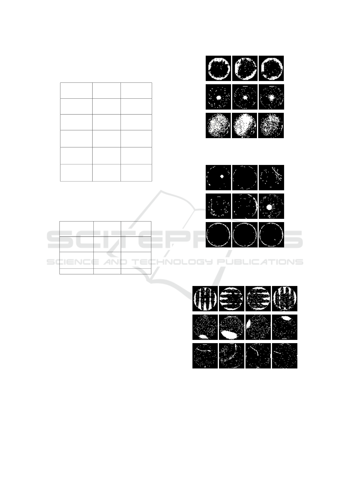
Table 2: Clustering outcomes when changing clustering al-
gorithm and EWS maps descriptor (LBP: Local Binary Pat-
tern, PCs: Principal Components). Precision is computed
as T P/(T P + FP). The best result is highlighted in bold.
Clustering Descriptor Precision %
KMeans LBP 48.98
KMeans PCs 70.6
Hierarchical
clustering
divisive
LBP 58.44
Hierarchical
clustering
divisive
PCs 79.05
Hierarchical
clustering
aggregative
PCs 90.20
Table 3: Classification outcomes comparing K-Nearest
Neighbours (KNN) and Convolutional Neural Network
(CNN). EWS maps selected descriptors are the Principal
Components (PCs). Precision is computed as T P/(T P +
FP). The best result is highlighted in bold.
Classification Descriptor Precision %
KNN PCs 85.33
KNN with
affinity
percentage
PCs 90.55
CNN PCs 95.87
nificantly increases the processing time to few hours a
day, which makes it not feasible for real use-cases in-
dustrial applications. Another good quality of the pro-
posed method is its proved rotation invariance (Fig-
ure 5).
Classification outcomes are reported in Table 3.
KNN is proved to be good enough for classification
purposes, reaching more than 90% of precision. As
expectable, CNN was able to improve this result,
reaching 95.87% of precision. Since we are deal-
ing with skewed data, we also computed for CNN
the more robust F1-score, that is equal to 92.18%.
Considering we started from a not labeled dataset,
our results sound comparable with the ones shown
in (Saqlain et al., 2019), where they obtained 96.93%
of precision and 96.71% of F1-score with only 9
classes (WM-811K, 2018), instead of the 85 em-
ployed in this work.
Figure 3: Three clusters (one per row) obtained through K-
Means and Principal Components (PCs). This is an example
of good clustering.
Figure 4: Three clusters (one per row) obtained through
divisive hierarchical clustering and Local Binary Pattern
(LBP). This is an example of bad clustering: first and sec-
ond clusters contains different kind of anomalies signatures.
Only the third cluster looks fine.
Figure 5: Proposed clustering method is proved to be rota-
tion invariant.
4 CONCLUSION
In this work, we focused onto a very specific kind of
data from semiconductor manufacturing called Elec-
Semisupervised Classification of Anomalies Signatures in Electrical Wafer Sorting (EWS) Maps
283

trical Wafer Sorting (EWS) maps. These images are
generated during the wafer testing phase performed
in semiconductor device fabrication. We assumed to
handle binary EWS maps, where white pixels identify
failed dies, while black pixels the good ones. Usually,
yield detractors are identified by specific and charac-
teristic patterns, named anomalies signatures. These
patterns are useful for investigating the root causes
that could be, for instance, related to an equipment
component failure, a drifting process, or an integra-
tion of processes (May and Spanos, 2006). Unfortu-
nately, new anomalies signatures may appear among
the huge amount of EWS maps generated per day.
Hence, it’s unfeasible to define just a finite set of pos-
sible signatures, as this will not represent a real use-
case scenario. For the same reason, we did not gath-
ered a labeled dataset.
In this paper, we presented a new semisupervised
approach for classifying anomalies signatures in EWS
maps, by combining an unsupervised approach using
a Hierarchical clustering algorithm to create the start-
ing Knowledge base, and a supervised one through
a classifier trained leveraging clustering phase. The
knowledge base represents our core knowledge about
the possible anomalies signatures (i.e., the number of
clusters) known until each daily update. We therefore
dynamically proceeded to test our clustering proce-
dure on the incrementing dataset. Indeed, our dataset
can be daily increased, and the classifier is dynami-
cally updated considering possible new created clus-
ters. The workflow of our solution can be resumed in:
daily arrival of EWS maps, clustering of newcomer
images into previously created clusters, possible cre-
ation of new clusters, anomalies signatures classifica-
tion.
We compared several clustering and classifica-
tion techniques. We found that aggregative hierarchi-
cal clustering leveraging Principal Components com-
puted through the Principal Component Analysis can
be a robust clustering method. Then, we trained a
Convolutional Neural Network with ResNet-18 archi-
tecture, reaching performance comparable with other
state-of-the-art technique. We remark that our method
does not rely on any labeled dataset and can be daily
updated, differently by compared literature. Our
dataset is skewed, a common characteristic in real
use-case industrial scenario. Moreover, we proposed
a method that was proved to be rotation invariant.
The goal of this work was to create a tool to make
as automatic as possible the recognition of wafer
anomalies signatures. This is meaningful as upon
classification the industrial system can be able to au-
tomatically choose (or at least suggest) either to dis-
card a wafer or to ship it to the customer. The pro-
posed method can also grant benefits like reduction
of wafer test results review time, or improvement of
processes, yield, quality, and reliability of production
using the information obtained during clustering pro-
cess.
As future works, we are planning to investigate
performance of other CNN architectures. We are also
designing a comparison study with a two-fold pur-
pose: consolidate outcomes shown in this proposal
employing the WM-811K dataset, and exploring the
existence of any correlation with test phases before
the EWS (e.g., relatively to Wafer Defect Maps -
WDM).
REFERENCES
Ackermann, M. R., Bl
¨
omer, J., Kuntze, D., and Sohler, C.
(2014). Analysis of agglomerative clustering. Algo-
rithmica, 69(1):184–215.
Balcan, M.-F., Liang, Y., and Gupta, P. (2014). Robust hier-
archical clustering. The Journal of Machine Learning
Research, 15(1):3831–3871.
Bryant, D. and Berry, V. (2001). A structured family of
clustering and tree construction methods. Advances in
Applied Mathematics, 27(4):705–732.
Di Bella, R., Carrera, D., Rossi, B., Fragneto, P., and Bo-
racchi, G. (2019). Wafer defect map classification us-
ing sparse convolutional networks. In International
Conference on Image Analysis and Processing, pages
125–136. Springer.
Hadid, A., Zhao, G., Ahonen, T., and Pietik
¨
ainen, M.
(2008). Face analysis using local binary patterns. In
Handbook of Texture Analysis, pages 347–373. World
Scientific.
Han, J., Kamber, M., and Tung, A. K. (2001). Spatial clus-
tering methods in data mining. Geographic data min-
ing and knowledge discovery, pages 188–217.
He, K., Zhang, X., Ren, S., and Sun, J. (2015). Deep
residual learning for image recognition. CoRR,
abs/1512.03385.
Jin, C. H., Na, H. J., Piao, M., Pok, G., and Ryu, K. H.
(2019). A novel dbscan-based defect pattern detection
and classification framework for wafer bin map. IEEE
Transactions on Semiconductor Manufacturing.
Li, Z. and de Rijke, M. (2017). The impact of linkage
methods in hierarchical clustering for active learning
to rank. In Proceedings of the 40th International ACM
SIGIR Conference on Research and Development in
Information Retrieval, pages 941–944. ACM.
May, G. S. and Spanos, C. J. (2006). Fundamentals of semi-
conductor manufacturing and process control. Wiley
Online Library.
Mishra, S. P., Sarkar, U., Taraphder, S., Datta, S., Swain,
D. P., Saikhom, R., Panda, S., and Laishram, M.
(2017). Multivariate statistical data analysis-principal
component analysis (pca). International Journal of
Livestock Research, 7(5):60–78.
VISAPP 2020 - 15th International Conference on Computer Vision Theory and Applications
284

Murtagh, F. and Legendre, P. (2014). Ward’s hierarchical
agglomerative clustering method: which algorithms
implement ward’s criterion? Journal of classification,
31(3):274–295.
Saqlain, M., Jargalsaikhan, B., and Lee, J. Y. (2019). A
voting ensemble classifier for wafer map defect pat-
terns identification in semiconductor manufacturing.
IEEE Transactions on Semiconductor Manufacturing,
32(2):171–182.
Thinsungnoena, T., Kaoungkub, N., Durongdumronchaib,
P., Kerdprasopb, K., and Kerdprasopb, N. (2015). The
clustering validity with silhouette and sum of squared
errors. learning, 3:7.
Tsigkritis, T., Groumas, G., and Schneider, M. (2018). On
the use of k-nn in anomaly detection. Journal of In-
formation Security, pages 635–645.
Turk, M. and Pentland, A. (1991). Eigenfaces for recogni-
tion. Journal of cognitive neuroscience, 3(1):71–86.
Tvaronaviciene, M., Razminiene, K., and Piccinetti, L.
(2015). Aproaches towards cluster analysis. Eco-
nomics & sociology, 8(1):19.
Wang, M., Abrams, Z. B., Kornblau, S. M., and Coombes,
K. R. (2018). Thresher: determining the number of
clusters while removing outliers. BMC bioinformat-
ics, 19(1):9.
WM-811K (2018). Wafer Maps Image dataset available
on Kaggle. https://www.kaggle.com/qingyi/
wm811k-wafer-map. Online; last visited 09/19.
Wu, M.-J., Jang, J.-S. R., and Chen, J.-L. (2014). Wafer
map failure pattern recognition and similarity ranking
for large-scale data sets. IEEE Transactions on Semi-
conductor Manufacturing, 28(1):1–12.
Xu, S., Qiao, X., Zhu, L., Zhang, Y., Xue, C., and Li, L.
(2016). Reviews on determining the number of clus-
ters. Applied Mathematics and Information Sciences,
10(4):1493–1512.
Zhang, W., Li, X., Saxena, S., Strojwas, A., and Rutenbar,
R. (2013). Automatic clustering of wafer spatial sig-
natures. In Proceedings of the 50th Annual Design
Automation Conference, page 71. ACM.
Semisupervised Classification of Anomalies Signatures in Electrical Wafer Sorting (EWS) Maps
285