
Exploiting Bilateral Symmetry in Brain Lesion Segmentation with
Reflective Registration
Kevin Raina
a
, Uladzimir Yahorau
b
and Tanya Schmah
c
Department of Mathematics and Statistics, University of Ottawa, Ontario, Canada
Keywords:
Stroke, Brain Lesions, Lesion Mapping, Image Segmentation, MRI, Convolutional Neural Network.
Abstract:
Brain lesions, including stroke lesions and tumours, have a high degree of variability in terms of location,
size, intensity and form, making automatic segmentation difficult. We propose an improvement to existing
segmentation methods by exploiting the bilateral quasi-symmetry of healthy brains, which breaks down when
lesions are present. Specifically, we use nonlinear registration of a neuroimage to a reflected version of itself
(“reflective registration”) to determine for each voxel its homologous (corresponding) voxel in the other hemi-
sphere. A patch around the homologous voxel is added as a set of new features to the segmentation algorithm.
To evaluate this method, we implemented two different CNN-based multimodal MRI stroke lesion segmenta-
tion algorithms, and then augmented them by adding extra symmetry features using the reflective registration
method described above. For each architecture, we compared the performance with and without symmetry
augmentation, on the SISS Training dataset of the Ischemic Stroke Lesion Segmentation Challenge (ISLES)
2015 challenge. Using linear reflective registration improves performance over baseline, but nonlinear reflec-
tive registration gives significantly better results: an improvement in Dice coefficient of 13 percentage points
over baseline for one architecture and 9 points for the other. We argue for the broad applicability of adding
symmetric features to existing segmentation algorithms, specifically using the proposed nonlinear, template-
free method.
1 INTRODUCTION
Segmentation of lesions in neuroimages, also called
lesion mapping, can give valuable information for
prognosis, treatment planning and monitoring of dis-
ease progression. The “gold standard” for lesion seg-
mentation is still manual delineation by a human ex-
pert, going through each of the horizontal slices of
the three-dimensional image and labeling each sepa-
rate voxel as either healthy or belonging to a lesion.
This is tedious, time-consuming, and often imprac-
tical, and therefore in practice, a human expert usu-
ally gives only a qualitative assessment of lesions.
Further, there is inter-observer variability; the size
of this variability varies significantly by task, but we
note that an average Dice score of 0.58 for overlap
of manually-outlined lesions by two raters was re-
ported for the ISLES2016 challenge (Winzeck et al.,
2018). These observations indicate a need for auto-
matic brain lesion segmentation algorithms. How-
a
https://orcid.org/0000-0002-6240-9675
b
https://orcid.org/0000-0002-0522-4148
c
https://orcid.org/0000-0002-0404-8824
ever, accurate lesion segmentation is a challenging
task for many reasons, including large variability in
location, size, shape and frequency of lesions across
patients.
While a plethora of automatic lesion segmenta-
tion methods has been proposed, most of the currently
leading methods are based on convolutional neural
networks (CNN) (Winzeck et al., 2018). Many of
these use 2D CNNs, where the 3D neuroimage is pro-
cessed as a sequence of independent 2D slices. These
approaches are arguably suboptimal, since they do not
take into account the 3D spatial structure of the data.
Nonetheless, many 2D methods have shown promis-
ing results, including the methods of Havaei et al.
(Havaei et al., 2017) and Kamnitsas et al. (Kamnitsas
et al., 2017), which we use as baseline architectures in
the present paper. Some other works have used CNNs
with an input of three orthogonal patches around each
voxel being classified, thus incorporating some 3D in-
formation, however this significantly increased mem-
ory requirements and computational complexity. The
technique of dense inference greatly sped up infer-
ence time, and led to several successful 3D segmenta-
tion methods, see discussion and references in Kam-
116
Raina, K., Yahorau, U. and Schmah, T.
Exploiting Bilateral Symmetry in Brain Lesion Segmentation with Reflective Registration.
DOI: 10.5220/0008912101160122
In Proceedings of the 13th International Joint Conference on Biomedical Engineering Systems and Technologies (BIOSTEC 2020) - Volume 2: BIOIMAGING, pages 116-122
ISBN: 978-989-758-398-8; ISSN: 2184-4305
Copyright
c
2022 by SCITEPRESS – Science and Technology Publications, Lda. All rights reserved

nitsas et al. (Kamnitsas et al., 2017).
We propose a general method for improving ex-
isting segmentation algorithms, including all of the
CNN-based methods mentioned above, by exploit-
ing the bilateral quasi-symmetry of healthy brains.
This symmetry often breaks down when lesions are
present. In particular, stroke lesions usually affect
only one hemisphere; while for some other lesion
types such as tumours, lesions may be present in both
hemispheres but any symmetry is coincidental and
rare. The basic idea is illustrated in Figure 1. The
first subfigure shows an axial slice of a brain with a
stroke lesion in one hemisphere, and two homologous
(“mirror”) voxels, i.e voxels in corresponding parts
of the brain but in opposite hemispheres. Through-
out this paper, homologous voxels are determined us-
ing “reflective registration”, which is registration of
an image to its own reflection, as detailed in the next
section. In healthy normal brains, there is a strong
correlation between intensities of homologous vox-
els. In lesioned brains, voxels in a lesion often have
intensities very different from the intensities of their
homologous voxels, as shown in Fig. 1 (b). On the
other hand, lesions typically represent a small propor-
tion of total brain volume, so non-lesion voxels typi-
cally have non-lesion mirror voxels as well, typically
resulting in small intensity differences (if the mirror
voxels have been accurately located). The distribu-
tion of these intensity differences, for both lesion and
non-lesion voxels, is illustrated in Figures 1 (c) and
(d). The difference between these two subfigures is in
the nature of the reflective registration used to iden-
tify homologous voxels: in (c), “linear” (affine) reg-
istration is used, while in (d), nonlinear registration
is used. The increase in mass around zero for non-
lesions when using nonlinear registration (d) in com-
parison to linear registration (c) suggests the supe-
riority of nonlinear reflective registration in locating
mirror voxels. In both cases, the pattern of intensity
differences can be used to aid the classification of a
voxel as lesion or non-lesion. This method is inspired
by the clinical practice of radiologists, who make fre-
quent use of comparisons with homologous areas to
detect abnormalities.
Our method, explained in more detail below, uses
3D nonlinear registration of a neuroimage with a re-
flected version of itself to determine for each voxel its
homologous voxel in the other hemisphere. A patch
around the homologous voxel is added as a set of
new features to the segmentation algorithm. To eval-
uate this method, we implemented two baseline mul-
timodal MRI stroke lesion segmentation algorithms,
both based on 2D CNNs, following Havaei et al.
(Havaei et al., 2017) and Kamnitsas et al. (Kamnit-
sas et al., 2017), and then augmented them by adding
extra symmetry features as described above. For each
architecture, we evaluated the baseline method and
two versions of symmetry augmentation: one using
“linear” (affine) registration only, and one using non-
linear registration. We compared the performance of
these three segmentation methods on the SISS Train-
ing dataset of the Ischemic Stroke Lesion Segmen-
tation Challenge (ISLES 2015)(Maier et al., 2017).
Though our experiments use 2D CNNs, our method
can be applied without modification to 3D CNNs.
We are aware of three prior works that have also
used brain quasi-symmetry to improve the perfor-
mance of CNN based methods: (Shen et al., 2017),
(Wang et al., 2016) and (Zhang et al., 2017). Shen
et al. use the SIFT-based method of Loy and Eklundh
(Loy and Eklundh, 2006) to identify homologous vox-
els, and report a mean improvement of 3% in Dice
scores on the high-grade (HG) BraTS2013 (brain tu-
mor) Training set. Wang et al. report a higher in-
crease in mean Dice scores, from 0.63 to 0.78, on
a private test set of 8 brains with chronic stroke le-
sions. However the method they use is unclear; the
absence of such an explanation suggests a simple lin-
ear transformation, perhaps a reflection in the medial
(mid-sagittal) plane. Zhang et al. uses a reflection
in the medial plane of images that have already been
registered to a template (with the registration method
unspecified). Evaluations on the BraTS2017 dataset
show that adding symmetry features speeds conver-
gence of the algorithm, however there is no consis-
tent improvement in segmentation accuracy. All three
methods require homologous voxels to be in the same
axial plane, a restriction that our method does not
have.
We note that the idea of using symmetry also
appeared in early literature, prior to the widespread
use of neural networks, for example in (Meier et al.,
2014), (Schmidt et al., 2005) and (Dvorak et al.,
2013). These works are based on an initial linear reg-
istration of each subject’s brain to a template. This
is also true of (Tustison et al., 2015), with the ma-
jor differences being the use of multiple modalities
and nonlinear registration. Our contributions are thus
two-fold: (1) Using template-free registration of an
image with a reflected version of itself, called reflec-
tive registration, to produce supplementary features
for use by segmentation algorithms; and (2) demon-
strating that nonlinear reflective registration is better
than linear reflective registration for locating mirror
voxels, as judged by improved segmentation results.
Exploiting Bilateral Symmetry in Brain Lesion Segmentation with Reflective Registration
117
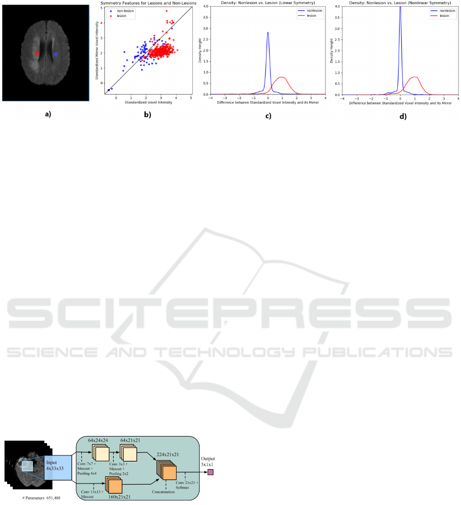
Figure 1: The quasi-symmetry property of the normal brain can be used to aid lesion segmentation. Subfigure (a) shows a
lesion voxel (red) and its non-lesion (blue) mirror voxel (projected onto the same axial slice); (b) shows the voxel intensity
plotted against the intensity of its mirror for a sample of 600 voxels taken from the same brain and equally divided between
lesions and non-lesions; (c) and (d) show superimposed densities for the difference between standardized intensities of a
voxel and its mirror, based on a sample of 2000 voxels taken from the same brain and equally divided amongst lesions and
non-lesions, where homologous voxels have been identified using linear and nonlinear reflective registration in (c) and (d)
respectively.
2 METHODS
Our two baseline algorithms are slight modifications
of: (i) TwoPathCNN by Havaei et al. (Havaei et al.,
2017), see Figure 2; and (ii) Wider2dSeg by Kamnit-
sas et al. (Kamnitsas et al., 2017). All of the 2D archi-
tectures in Kamnitsas et al. (Kamnitsas et al., 2017),
including Wider2dSeg, are two dimensional variants
of their 3D deepMedic architecture. The 2D archi-
tectures vary in the number of layers, feature maps
(FMs) per layer, and FMs per hidden layer. See Table
B.1 in Appendix B of Kamnitsas et al. (Kamnitsas
et al., 2017) for more details. We first describe the ar-
chitectures and training of these baseline models, and
then describe how to compute and append symmet-
ric features so as to preserve dense inference on 2D
images of arbitrary size.
Figure 2: TwoPathCNN architecture, reproduced from
Havaei et al. (Havaei et al., 2017) with permission of the
authors. Note that the final output is a 2 × 1 × 1 tensor for
our application.
2.1 Baseline Models
TwoPathCNN and Wider2dSeg are convolutional
neural networks. Both architectures take as input
one or, as in the case of Kamnitsas’ 2D architec-
tures, two stacks of four patches from different MRI
modalities. The networks branch into two path-
ways. TwoPathCNN consists of three convolutional
blocks of sizes shown in Fig. 2, which also shows
the locations of maxout and max pooling operations.
Wider2dSeg is a deeper architecture with 16 convo-
lutional blocks that makes use of multiscale features
through downsampling, convolution and upsampling
back to the original scale. This allows for a larger area
of information to be used. For more details on the ar-
chitectures, see (Havaei et al., 2017) and (Kamnitsas
et al., 2017). An important feature of these architec-
tures is that all the layers of the network are convo-
lutional, enabling dense inference on full images or
image segments.
2.1.1 Training
We interpret the output of the CNNs as predicted la-
bel probabilities for lesion, and define a training loss
function consisting of the negative log likelihood with
both L1 and L2 regularization. This loss is minimised
by following a stochastic gradient descent approach
on randomly selected minibatches of patches within
each brain.
Performance of CNNs depends greatly on the dis-
tribution of the training samples. A commonly used
approach is to train a classifier on the same number
of image patches from each of the classes per mini-
batch. However since the classes are imbalanced, this
approach biases the classifier towards making false
positive predictions.
In TwoPathCNN, we follow the two-phase train-
ing proposed in [3] with minibatches of one labeled
sample per training instance. In the first phase, the
mini-batches are equally divided among lesions and
BIOIMAGING 2020 - 7th International Conference on Bioimaging
118

backround. In the second phase, we keep the weights
of all layers fixed and retrain only the final layer on
patches uniformly extracted to be closer to the true
data distribution.
For Wider2dSeg, the patch size fed down each
pathway is larger than the network’s receptive field
(Kamnitsas et al., 2017). This technique, called dense
training, increases the effective batch size by con-
structing mini-batches of more than one labeled sam-
ple per training instance since it allows the network
to segment a neighborhood of voxels sorrounding the
central voxel. (Kamnitsas et al., 2017). This makes
the patch size, also called image segment size, an im-
portant parameter to tune since larger patch sizes cap-
ture more background voxels than smaller patch sizes.
2.2 Implementation Details
We implemented the models using Tensorflow (Abadi
et al., 2016). We apply only minimal pre-processing:
we normalize within each input channel by subtract-
ing its mean and dividing by its standard deviation.
Unlike (Havaei et al., 2017), we did not use N41TK
bias correction and we did not remove the 1% highest
and lowest intensities. Similarily we didn’t use batch
normalization as proposed in (Kamnitsas et al., 2017)
since it is more of a requirement for 3D architectures.
We use standard momentum and fix the momentum
coefficient µ = 0.6 throughout training for all archi-
tectures.
2.2.1 TwoPathCNN
Weights are initialized from a uniform distribution on
(−0.005, 0.005), as in (Havaei et al., 2017), and bi-
ases are initialized to zero. Every epoch consists of
10,000 iterations of stochastic gradient descent with
momentum on mini-batches of 10 labeled samples.
Each sample consists of 4 stacked patches of size
33 × 33, each patch correspond to a different MRI
modality, and a label, which is the ground truth la-
bel for the central voxel in the patch. The first phase
of training consists of 50,000 iterations or 5 epochs.
The minibatches at this stage contain equal number of
positive and negative examples. The learning rate is
set to 0.001 decays by a factor of 0.1 (Havaei et al.,
2017) starting from the third epoch. The second phase
of training consists of another 4 epochs of 10,000 it-
erations each. The minibatches at this stage have the
property that approximately 2% of samples presented
in them are labeled as negative. The learning rate is
reset to 0.001 and decays by a factor of 0.1 after each
epoch. Thus, in total, the model is trained on 900,000
samples. The L
1
regularization constant is 10
−6
and
the L
2
regularization constant is 10
−4
. For further
regularization, dropout at a rate of 0.5 was applied on
hidden layers of the local pathway. In all of these im-
plementation details, we follow (Havaei et al., 2017),
except that the regularization constants were inspired
from (Kamnitsas et al., 2017) (which used the same
dataset as we do), but changed to account for the in-
creased number of parameters.
2.2.2 Wider2dSeg
As in (Kamnitsas et al., 2017), we use the weight ini-
tiliazation method of He et al. (He et al., 2015), since
deeper architectures are prone to larger signal vari-
ance. The bias terms are initialized to zero. We used
the RMSProp optimizer for a total of 80,000 iterations
with a learning rate of 0.001 and decayed it by a factor
of 0.5 (Kamnitsas et al., 2017) at the the following it-
erations: 25,000, 39,000, 49,000, 59,000, 71,000, and
75,000. In contrast to (Kamnitsas et al., 2017), we
use an image segment size of 43 for the first pathway
and 75 for the second pathway, which segments the
27
2
neighborhood around the central voxel per train-
ing instance. Mini-batches are of size 12 and equally
divided amongst lesions and background. The batch
and image segment sizes were chosen to achieve the
same effective batch size shown in Table B.1 of Ap-
pendix B from (Kamnitsas et al., 2017). To regularize
the network we follow (Kamnitsas et al., 2017) and
set the L
1
constant to 10
−8
, the L
2
constant to 10
−6
,
and apply dropout at a rate of 0.5 on the last two hid-
den layers.
2.3 Symmetry-augmented Methods
(LSymm and NLSymm)
For each subject, we augment the four image modali-
ties by four “mirror” images produced as follows. We
begin by producing a reflected FLAIR image by re-
versing the orientation of the x (left-right) axis, using
the fslorient tool of FSL (Smith et al., 2001). Since
the original images are linearly co-registered, this step
is approximately a reflection in the median, i.e. mid-
sagittal, plane. (FLAIR was chosen due to its frequent
use in lesion segmentation, however we intend in later
work to compare the use of T1 or multiple modali-
ties in this step.) We align the result with the original
FLAIR image using either “linear”/affine (LSymm) or
nonlinear (NLSymm) registration. This step uses the
SynQuick method in the ANTs package (Avants et al.,
2009). For LSymm, the “-t a” option was used, giv-
ing a 2-stage rigid+affine registration. For NLSymm,
the default options were used, giving a 3-stage rigid +
affine + nonlinear (“SyN”) registration. In either case,
the resulting transformation, composed with a reflec-
Exploiting Bilateral Symmetry in Brain Lesion Segmentation with Reflective Registration
119
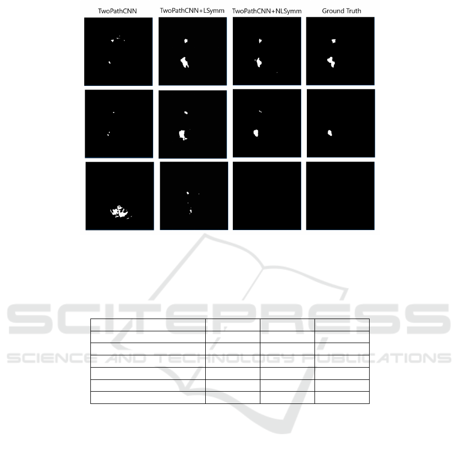
Figure 3: An example of different segmentations of Brain #8 of the SISS2015 Training set from the ISLES2015 Chal-
lenge. From left to right, the columns show segmentations produced by the TwoPathCNN, TwoPathCNN+LSymm and
TwoPathCNN+NLSymm methods, and the ground truth.
Table 1: Performance of TwoPathCNN and Wider2dSeg based on a 7-fold cross-validation for baseline, NLSymm and LSymm
on the ISLES2015 (SISS) training data. Results for Dice, Recall and Precision (Havaei et al., 2017) are shown as mean (std.
dev.).
Architecture Dice Recall Precision
TwoPathCNN 0.45(0.25) 0.59(0.22) 0.45(0.29)
TwoPathCNN+LSymm 0.52(0.23) 0.63(0.23) 0.50(0.28)
TwoPathCNN+NLSymm 0.54(0.21) 0.65(0.22) 0.52(0.26)
Wider2dSeg 0.49(0.25) 0.53(0.28) 0.54(0.25)
Wider2dSeg+LSymm 0.61(0.22) 0.58(0.25) 0.67(0.22)
Wider2dSeg+NLSymm 0.62(0.22) 0.60(0.25) 0.68(0.21)
tion, produces a symmetry transformation T (x, y, z)
that associates to each voxel its corresponding “mir-
ror” voxel in the opposite hemisphere.
Once we have obtained our linear or nonlinear
symmetry transformation for each subject, we use it
to construct a Symmetry Difference Image for each
modality, by subtracting from each voxel’s standard-
ized intensity the standardized intensity of the “mir-
ror” voxel, S
r
(x, y, z) = I
r
(x, y, z) − I
r
(T (x, y, z)).
This results in 4 Symmetry Difference Images
(SDIs), one for each modality, which we use to aug-
ment the original 4 images. For instance in the base-
line TwoPathCNN model, for each voxel, one 33×33
patch is extracted from each of the 4 MR images and
combined into a 4 × 33 × 33 tensor; in LSymm and
NLSymm, one 33 × 33 patch is extracted from each
of the 8 MR images (originals plus SDIs) and com-
bined into a 8 × 33 × 33 tensor. This double-size ten-
sor is fed into the both the local and global pathways
of the TwoPathCNN architecture. Apart from dou-
bling the number of images from 4 to 8, all details of
architecture and training are exactly as in the baseline
methods.
3 EXPERIMENTAL RESULTS
3.1 Dataset
We evaluated our methods on the ISLES2015 (SISS)
training data. The training data consists of FLAIR,
DWI ,T1 and T1-contrast images of size 230 × 230 ×
154, for each of 28 patients with sub-acute ischemic
stroke lesions. All images are skull-stripped and have
isotropic 1mm
3
voxel resolution.
BIOIMAGING 2020 - 7th International Conference on Bioimaging
120

3.2 Experiment
For each of the two architectures, we compare the
three methods described above: baseline, baseline
with LSymm, and baseline with NLSymm, using 7-
fold cross-validation on the Training dataset of 28
subjects. All methods are run with the same hyper-
parameters, on the same pseudo-random sequence of
training patches.
3.3 Results
Example segmentations produced by the three meth-
ods on TwoPathCNN are shown in Fig. 3. The main
results are summarised in Table 1. Adding linearly or
nonlinearly registered symmetry features (LSymm or
NLSymm) to the baseline architectures consistently
improves mean Dice coefficient, Recall and Precision,
showing the effectiveness of reflective registration.
For the Dice coefficient, we performed one-sided
paired t-tests for symmetry-augmented vs. baseline
methods, and found that the resulting p-values were
always less than 10
−5
, for both LSymm and NLSymm
and for both baseline architectures. Moreover, nonlin-
early registered symmetry features (NLSymm) con-
sistently produced higher Dice, Recall and Precision
scores compared to linearly registered symmetry fea-
tures (p < 0.001 for the TwoPathCNN architecture,
and p = 0.08 for the Wider2dSeg architecture). Of
the two architectures evaluated, Wider2dSeg benefit-
ted more from the symmetry augmentation, however
the difference between LSymm and NLSymm was
not significant; both differences were perhaps due to
its deeper architecture.
4 CONCLUSIONS
We have proposed an improvement to existing seg-
mentation methods by exploiting the bilateral quasi-
symmetry of healthy brains. Our method, which does
not require a template, consists of augmenting the in-
put images to a CNN with extra Symmetry Difference
Images, which are intensity differences between ho-
mologous (“mirror”) voxels in different hemispheres.
We showed how to incorporate these symmetric fea-
tures into the increasingly popular patch-based CNNs
so as to preserve dense inference. In an experi-
ment on the ISLES2015 SISS dataset, we found that
adding symmetric features generated using nonlinear
reflective registration (the “NLSymm” method) con-
sistently resulted in a mean improvement in Dice co-
efficient, Recall and Precision. Using linear reflec-
tive registration instead gave consistently smaller im-
provements over baseline, showing that nonlinear reg-
istration is superior in this application. For the Dice
coefficient, improvement over baseline was signifi-
cant (p < 10
−5
) for both linear and nonlinear sym-
metric features. The nonlinear method was signifi-
cantly better than the linear one (p < 0.001) for one
baseline architecture (TwoPathCNN) but not the other
(Wider2dSeg).
While our numerical results are not directly com-
parable with those of the three preceding studies of
symmetric feature augmentation for CNNs mentioned
in the Introduction, we note that our improvements in
Dice scores of 9 to 13% on an open dataset compare
favourably to earlier results.
We have shown that the brain’s quasi-symmetry
property is a valuable tool for brain lesion segmenta-
tion. The ease of application of symmetry augmen-
tation to most existing CNN methods and many other
methods suggests a potentially wide-ranging utility of
the method.
REFERENCES
Abadi, M., Barham, P., Chen, J., Chen, Z., Davis, A., Dean,
J., Devin, M., Ghemawat, S., Irving, G., Isard, M.,
et al. (2016). Tensorflow: a system for large-scale
machine learning. In OSDI, volume 16, pages 265–
283.
Avants, B. B., Tustison, N. J., Song, G., and Gee, J. C.
(2009). ANTS: Open-source tools for normalization
and neuroanatomy. Transac Med Imagins Penn Image
Comput Sci Lab.
Dvorak, P., Bartusek, K., and Kropatsch, W. (2013). Au-
tomated segmentation of brain tumour edema in flair
mri using symmetry and thresholding. PIERS Pro-
ceedings, Stockholm, Sweden.
Havaei, M., Davy, A., Warde-Farley, D., Biard, A.,
Courville, A., Bengio, Y., Pal, C., Jodoin, P.-M., and
Larochelle, H. (2017). Brain tumor segmentation
with deep neural networks. Medical image analysis,
35:18–31.
He, K., Zhang, X., Ren, S., and Sun, J. (2015). Delv-
ing deep into rectifiers: Surpassing human-level per-
formance on imagenet classification. In Proceedings
of the IEEE international conference on computer vi-
sion, pages 1026–1034.
Kamnitsas, K., Ledig, C., Newcombe, V. F., Simpson,
J. P., Kane, A. D., Menon, D. K., Rueckert, D., and
Glocker, B. (2017). Efficient multi-scale 3D CNN
with fully connected CRF for accurate brain lesion
segmentation. Medical image analysis, 36:61–78.
Loy, G. and Eklundh, J.-O. (2006). Detecting symmetry
and symmetric constellations of features. In Euro-
pean Conference on Computer Vision, pages 508–521.
Springer.
Maier, O., Menze, B. H., von der Gablentz, J., H
¨
ani, L.,
Heinrich, M. P., Liebrand, M., Winzeck, S., Basit, A.,
Exploiting Bilateral Symmetry in Brain Lesion Segmentation with Reflective Registration
121

Bentley, P., Chen, L., et al. (2017). ISLES 2015 - a
public evaluation benchmark for ischemic stroke le-
sion segmentation from multispectral MRI. Medical
image analysis, 35:250–269.
Meier, R., Bauer, S., Slotboom, J., Wiest, R., and Reyes, M.
(2014). Appearance-and context-sensitive features for
brain tumor segmentation. Proceedings of MICCAI
BRATS Challenge, pages 020–026.
Schmidt, M., Levner, I., Greiner, R., Murtha, A., and
Bistritz, A. (2005). Segmenting brain tumors us-
ing alignment-based features. In Fourth International
Conference on Machine Learning and Applications
(ICMLA’05), pages 6–pp. IEEE.
Shen, H., Zhang, J., and Zheng, W. (2017). Efficient
symmetry-driven fully convolutional network for mul-
timodal brain tumor segmentation. In 2017 IEEE In-
ternational Conference on Image Processing (ICIP),
pages 3864–3868. IEEE.
Smith, S., Bannister, P. R., Beckmann, C., Brady, M., Clare,
S., Flitney, D., Hansen, P., Jenkinson, M., Leibovici,
D., Ripley, B., et al. (2001). FSL: New tools for func-
tional and structural brain image analysis. NeuroIm-
age, 13(6):249.
Tustison, N. J., Shrinidhi, K., Wintermark, M., Durst, C. R.,
Kandel, B. M., Gee, J. C., Grossman, M. C., and
Avants, B. B. (2015). Optimal symmetric multimodal
templates and concatenated random forests for su-
pervised brain tumor segmentation (simplified) with
antsr. Neuroinformatics, 13(2):209–225.
Wang, Y., Katsaggelos, A. K., Wang, X., and Parrish, T. B.
(2016). A deep symmetry convnet for stroke lesion
segmentation. In 2016 IEEE International Conference
on Image Processing (ICIP), pages 111–115. IEEE.
Winzeck, S., Hakim, A., McKinley, R., Pinto, J. A., Alves,
V., Silva, C., Pisov, M., Krivov, E., Belyaev, M.,
Monteiro, M., et al. (2018). ISLES 2016 and 2017-
benchmarking ischemic stroke lesion outcome predic-
tion based on multispectral MRI. Frontiers in neurol-
ogy, 9.
Zhang, H., Zhu, X., and Willke, T. L. (2017). Seg-
menting brain tumors with symmetry. arXiv preprint
arXiv:1711.06636. NIPS ML4H Workshop 2017.
BIOIMAGING 2020 - 7th International Conference on Bioimaging
122
