Aerial Radar Target Classification using Artificial Neural Networks

Guy Ardon

1,2

, Or Simko

1,2

and Akiva Novoselsky

Department of Electrical & Computer Engineering, Ben-Gurion University of the Negev, Beersheba, Israel

ELTA Systems Ltd. Group & Subsidiary of Israel Aerospace Industries Ltd., Ashdod, 771020, Israel

Keywords: Aerial Radar Target Classification, Radar Cross Section (RCS), Time-Series Classification, Fully-Connected

Neural Networks, Empirical Mode Decomposition (EMD).

Abstract: In this paper, we propose a new algorithm for classification of aerial radar targets by using Radar Cross

Section (RCS) time-series corresponding to target detections of a given track. RCS values are obtained

directly from SNR values, according to the radar equation. The classification is based on analysing the

behaviour of the RCS time-series, which is the unique “fingerprint” of an aerial radar target. The classification

process proposed in this paper is based on training a fully-connected neural network on features extracted

from the RCS time-series and its corresponding Intrinsic Mode Functions (IMFs). The training is based on a

database containing RCS signatures of various aerial targets. The algorithm has been tested on a large and

diverse set of simulative flight trajectories, and its performance has been compared with that of several

different methods. We have found that the proposed neural network-based classifier performed better on our

database.

1 INTRODUCTION

Conventional uses of radar systems include detection

of targets through transmission of radio waves and re-

scattering of echoes from targets (Skolnik, 1962).

Radar systems, however, do not provide information

regarding the specific type of target which is detected.

In the past few decades, there has been an effort

to approach the problem of radar target recognition

(Herman & Moulin, 2002) – (Notkin et al., 2019).

Most of the works presented so far utilized Radar

Cross Section (RCS) of aerial targets for

classification. RCS values are not obtained directly

by the radar. In fact, the radar yields signal-to-noise

ratio (SNR) values, which can be transformed into

RCS values by using the radar equation. The RCS

signature of aerial targets depends on various factors,

such as the target’s unique geometry, size,

orientation, and reflectiveness, as well as on the

transmission frequency. RCS values can therefore

provide useful information regarding target

characteristics.

RCS measurements of aerial targets are strongly

dependent on the aspect angles (azimuth and

elevation), relative to the radar. These angles

determine where the radar beam hits the target. Since

different points on the target reflect the radar beam

differently, RCS values are characterized by large

variances, and even a slight change in one of the

aspect angles can cause large fluctuations.

Nevertheless, development of an aerial target

recognition capability is of great interest. There have

been several proposals to classify targets based on

various methods (Herman & Moulin, 2002),

(Molchanov et al., 2012), (Tian et al., 2015), (Notkin

et al., 2019).

The RCS time-series corresponding to an aerial

target track contains abundant information, which can

be used to characterise target types. However, RCS

time-series is non-stationary, which makes it difficult

to analyse. This calls for a comprehensive signal

processing analysis.

Empirical Mode Decomposition (EMD) is an

effective nonlinear signal processing technique for

adaptively representing non-stationary signals as a

sum of zero-mean components, known as Intrinsic

Mode Functions (IMF) (Huang et al., 1998). Since its

introduction, it has been used in various applications

(Colominas et al., 2014).

In this paper, we present a new method for

classifying aerial radar targets based on fully-

connected neural networks. Our algorithm utilizes a

database of RCS signatures of various types of aerial

targets, at a given resolution of aspect angles. Given

an observed flight track, and the corresponding RCS

136

Ardon, G., Simko, O. and Novoselsky, A.

Aerial Radar Target Classiﬁcation using Artiﬁcial Neural Networks.

DOI: 10.5220/0008911701360141

In Proceedings of the 9th International Conference on Pattern Recognition Applications and Methods (ICPRAM 2020), pages 136-141

ISBN: 978-989-758-397-1; ISSN: 2184-4313

time-series, we extract RCS signals corresponding to

the track, for all available targets in the database. RCS

signals are then decomposed into IMFs using EMD.

Features are then extracted from this set of RCS and

corresponding IMF signals. Finally, a fully-

connected neural network is trained with these

features to identify the observed target.

We compare the neural network-based classifier

with the K-Nearest Neighbour (KNN) classifier and

three classifiers that are based on time-series

similarity measures. In these types of classifiers, a

target can be identified by measuring the similarity

between the measured RCS signal, and RCS signals

of available targets in the database, corresponding to

the same flight track.

The paper is organized as follows: Section 2

describes the data preparation, and feature extraction

stages. Section 3 describes the proposed neural

network. Section 4 presents the results. Conclusions

are provided in section 5.

2 THE METHOD FOR

PREPARING RCS DATA FOR

THE CLASSIFIER

In this section, we present our method for preparing

the training and test data for the neural-network based

classifier.

In this work, we simulated a database that

contains RCS signatures for 8 different targets at two

aspect angles relative to the radar: azimuth ∈

0,360

∘

 , and elevation ∈90

∘

,90

∘

 at a given

resolution. The targets are indicated by the letters A,

B, C

, C

, D and E. Targets C

1-4

are four

different configurations of the same aircraft model,

which lead to mild changes in RCS signature.

In addition to the simulated database, we

simulated a radar tracker, and target trajectories. The

tracker provided us with the position and velocity of

the target, as well as the aspect angles (azimuth and

elevation), relative to the radar. Knowing these aspect

angles enabled us to extract the corresponding RCS

values by interpolating the database.

In each simulation of a target trajectory, we

obtained a time-series of RCS values. The RCS time-

series corresponding to the observed flight track is

given by

∈



, where  is the number of

consecutive RCS measurements for a given

trajectory

Since aspect angles obtained by the radar are not

accurate, we generated RCS sequences for each pair

of possible aspect angles. This is done for all targets

in the database. The set of possible RCS time-

sequences for each of the targets form a “dynamic

bank”. The dynamic bank is denoted by

∈



 is the number of RCS measurements for a given

trajectory. Since aspect angle estimation has inherent

error, we generate  possible RCS sequences for

each target corresponding to a resolution of 

possible aspect angles.  is the number of targets in

the database.

The RCS time-series of a target-track is generally

composed of low-frequency and high-frequency

components. The assumption is that the low

frequencies correspond to the observation angle and

measurement errors, while the higher frequencies are

related to the target’s geometry and aspect angles

relative to the radar (Tian et al., 2015). Therefore, the

rapidly varying components in the RCS time-series

can characterize the targets well.

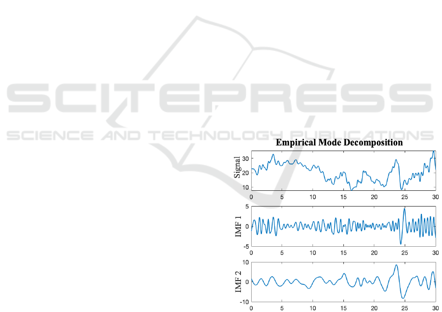
The RCS time-series is decomposed into

frequency components by using a signal processing

technique known as Empirical Mode Decomposition

(EMD). EMD decomposes a non-stationary signal

into stationary Intrinsic Mode Functions (IMFs)

(Huang et al., 1998; Rilling et al., 2003). The IMFs

are ordered according to their frequency components

from high to low, as shown in figure 1. By using the

temporal RCS data in the dynamic bank, and the

RCS time-series of the observed track  , we

implement EMD to decompose the RCS data into

IMFs.

Figure 1: EMD of a fluctuating signal into two intrinsic

mode functions.

At this stage, we extract ten features from the RCS

time-sequences in

, and ten features from their

corresponding IMFs. These features are later used as

training data for the neural network. The features are

chosen to characterize the statistical and spectral

Aerial Radar Target Classiﬁcation using Artiﬁcial Neural Networks

137

nature of the time sequences well, while at the same

time enabling separation of targets. Classifying

targets based on noisy radar data using these features

can suppress the effect the noise, in comparison with

classification based on the raw RCS data.

The first and second features, minimum and

maximum values, are used as a measure of the range

of values that the time-series can take. The next

feature is the number of zero-crossings, which can

represent the oscillatory nature of the signal. The next

four features; the mean, variance, skewness and

kurtosis of the time-series are the 1

-4

standardized

moments, where the sample mean is the average of

the time-series values, variance indicates the spread

of data from the mean, skewness is a measure of the

asymmetry of the data around the mean, and kurtosis

is a measure of how outlier-prone the distribution of

values is. The next feature is the energy of the signal,

which is the squared 



norm. The last two features

are Hjorth mobility and complexity (Hjorth, 1970).

Mobility represents the mean frequency, or the

portion of standard deviation of the power spectrum.

Hjorth complexity represents the change in frequency

of a signal.

The RCS and IMF features for each time-series in

the dynamic bank



are concatenated into the tensor:





∈







, where 



is number of elements in

each feature vector, and 

∙

 is the number of

training examples.  is the number of possible aspect

angles, and  is the number of targets in the database.

Each component in the feature vector is standardized

using the z-score normalization. The feature-tensor







has a corresponding label tensor:





∈





. We denote

,



as the ,  element in

the matrix, where 0,1,…,1 , and 

0,1, … ,   1.



,



1 if training example 

belongs to class , and 0 otherwise. The same feature

extraction process is applied to the signal  ,

corresponding to the observed target, with





∈







the corresponding feature vector, which will be

used to test the network.

3 THE PROPOSED NEURAL

NETWORK CLASSIFIER

In this section, we will describe the proposed neural

network-based classifier, and how it uses the features

to classify the aerial targets. Artificial neural

networks are mathematical models for solving

complex problems, originally inspired by the way in

which the brain processes information (Theodoridis

& Koutroumbas, 2003). The network is composed of

several layers of neurons, where the first layer is the

input layer, and the last layer is the network decision,

or solution to the problem. Neurons are nodes in the

network that take in a weighted sum of values and

produce a single output value, which is then

processed by more neurons in the next layer.

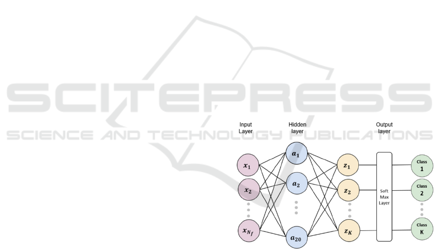
In order to identify the observed target as one of

the targets in the database, we use a 2-layer fully-

connected neural network. The network has one

hidden layer, and a softmax output layer that

normalizes the outputs into probabilities for each

target. The neurons in the hidden layer are defined by

a hyperbolic tangent activation function, which take

in a weighted sum of the values from the input layer,

and map the results to [-1,1]. We have found that the

network performs best when using one hidden layer,

with 20 neurons. Using fewer neurons led to poor

results, by being a too general solution, and using

more neurons, or more hidden layers, caused

overfitting the data.

In figure 2, the neural network architecture is

presented. The input layer has 



neurons,

corresponding to the number of features in each

feature-vector. The hidden layer’s neurons are

denoted by:



,



,…,



. The output layer has 

neurons, denoted by 



,



,…,



, which are

normalized in the softmax layer to obtain the final

outputs.

Figure 2: The proposed neural network architecture.

The neural network is trained on the feature

vectors in 





and the corresponding labels in





, as denoted in section 2. Training a neural

network consists of two stages, feedforward, and

backpropagation. Feedforward is the stage at which

outputs at each layer are fed towards the final output

layer. During backpropagation, we minimize a cross-

entropy loss function defining the error between the

desired values in





, and the network outputs at

the final layer. During the training process, the

weights are adjusted accordingly to give a better

ICPRAM 2020 - 9th International Conference on Pattern Recognition Applications and Methods

138

solution with each iteration. The weights and bias

values in each layer are optimized through scaled-

conjugate backpropagation (Møller, 1993).

The data was randomly split into training and

validation sets with a ratio of 80% - 20%

correspondingly. The training set was used to

compute the gradients, and update weights through

backpropagation. The validation set was used to

monitor the learning process. Both the training and

validation set errors are monitored during the training

process. At first, validation error decreases with the

training error, but after being presented with enough

data, the network starts to overfit to the training set,

the validation error begins to increase. We stop

updating the weights when the validation error is at a

minimum. In this way we make sure that the network

can generalize when presented with new examples.

Once the network is fully trained, we test the

network with





, the feature vector corresponding

to the RCS time-series of the observed target. The

network calculates probabilities for each target at the

output layer. Classification is defined as correct when

maximal probability corresponds to the correct target.

A pipeline figure for our algorithm is presented in

figure 3.

Figure 3: Dataflow and algorithm pipeline.

4 SIMULATION AND RESULTS

In this work, we simulated 640 target trajectories, 80

trajectories for each of the eight target types. The

classification accuracy of the neural network was

examined under various levels of noise. Additive

white Gaussian noise of up to 0.5

∘

was added to the

aspect angles of the target relative to the radar.

We defined a classification to be either be correct,

incorrect, or unknown. In order to reduce the false-

alarm rate, targets are defined to be ‘unknown’ when

there isn’t a good match in the database, or due to a

lack of data for a proper classification procedure. In

other words, it is better to define a target as

‘unknown’ than to classify it as an incorrect target.

For example, for a short flight track with few RCS

measurements, the features described in section 2

provide little value, and therefore we classify the

target as unknown.

Table 1 presents the confusion matrix for the 640

trajectories under 0.5

∘

of aspect angle noise. For this

amount of noise, we achieved an accuracy of 80.1%.

The accuracies of the network under various levels of

noise is presented in Table 2.

Table 1: Confusion matrix for the neural network-based

classifier. Results are shown for trajectories with additive

white Gaussian noise of 0.5

Actual Target

Predicted

Target

A B C D E

0 1 0 2

15 2 0

16 18

270

11 6

2 0 8

0 0 1 0

Unknown 5 4 25 4 6

Table 2: Final neural network classification results for the

simulated trajectories.

Aspect Angle Noise Accuracy

No Noise 93.3%

0.1

87.5%

0.3

82.7%

0.5

80.1%

We compared the results of the neural network-

based classifier with 5 other classifiers. The first

classifier is the K-Nearest Neighbours (KNN)

classifier (Covert & Hart, 1967). We implemented

KNN with the Mahalanobis distance metric, which

weights the distance by the inverse covariance of each

Radar Data

(Target Position, Target Velocity, SNR)

RCS Estimation

Generation of a dyanmic bank of possible RCS time-

sequences for targets in the database

Empirical Mode Decomposition of RCS time-series into

Intrinsic Mode Functions

Feature Extraction

Neural Network Training and Classification

Predicted Target Type

Aerial Radar Target Classiﬁcation using Artiﬁcial Neural Networks

139

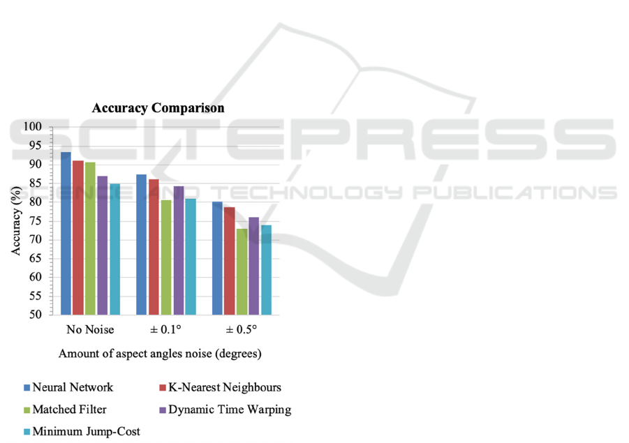
feature. We choose the target corresponding to the

minimum Mahalanobis distance as the correct target,

i.e. the first nearest neighbour.

The next three methods that we implemented take

a different approach, and rather than using features,

utilize time-series similarity measures between the

raw RCS signals in the dynamic bank and the RCS

signal of the observed target. The chosen target is the

target in the dynamic bank, with the most “similar”

RCS time-series. The first method used for time-

series similarity is the matched filter (Turin, 1960),

which correlates between signals by maximizing

SNR. The other two methods are Dynamic Time

Warping (Sakoe & Chiba, 1978), and Minimum

Jump-Cost (Serrà & Arcos, 2012), which work by

optimally aligning and stretching the time-series for

the best temporal match.

In figure 4, we compare the performance of the

proposed neural-network classifier with the other

methods. The performance of our proposed neural

network is better than the other methods.

Furthermore, the machine learning methods (neural

network and KNN) performed better under large

noise than the time-series similarity methods.

Figure 4: Classification accuracies for the compared

methods.

5 CONCLUSIONS

In this paper, we proposed a neural-network based

classifier for aerial radar targets. The classification is

based on features extracted from the RCS time-series

of an observed flight track and from its corresponding

IMFs. Comparison of the results have shown that our

classifier is better than other methods for the same

data. We conclude that the use of machine learning

can be effective for the task of aerial radar target

classification.

ACKNOWLEDGEMENTS

We would like to thank Ariel Rubanenko, Merav

Shomroni, Gregory Lukovsky, Nimrod Teneh, David

Feldman, and Or Livne for their useful discussion.

REFERENCES

Colominas, M.A., Schlotthauer, G. & Torres, M.E. (2014).

‘Improved complete ensemble EMD: A suitable tool for

biomedical signal processing’. Biomedical Signal

Processing and Control, 14, pp. 19-29.

Cover, T. & Hart, P. (1967). ‘Nearest Neighbor Pattern

Classification’. IEEE Transactions on Information

Theory, 13(1), pp.21-27.

Herman, S. & Moulin, P. (2002). ‘A particle filtering

approach to FM-band passive radar tracking and

automatic target recognition’, In: Proceedings, IEEE

Aerospace Conference, vol. 4, pp. 1789-1708.

Hjorth, B. (1970). ‘EEG analysis based on time domain

properties’. Electroencephalography and Clinical

Neurophysiology, 29(3), pp. 306-310.

Huang, N.E., Shen, Z., Long, S.R., Wu, M.C., Shih, H.H.,

Zheng, Q., Yen, N.C., Tung, C.C. & Liu, H.H. (1998).

‘The empirical mode decomposition and the Hilbert

spectrum for nonlinear and non-stationary time series

analysis’. In: Proceedings of the Royal Society of

London: Series A, 454(1971), pp. 903-995.

Molchanov, P, Totsky, A, Astola, J., Egiazarian, K.,

Leshchenko, S. & Rosa-Zurera, M. (2012). ‘Aerial

target classification by micro-Doppler signatures and

bicoherence-based features’. In: Proceedings of the 9th

European Radar Conference, pp. 214-217.

Møller, M.F. (1993). ‘A scaled conjugate gradient

algorithm for fast supervised learning’. In: Neural

Networks, 6(4), pp. 525-533.

Notkin, E. & Cohen, T. & Novoselsky, A. (2019).

‘Classification of Ground Moving Radar Targets with

RBF Neural Networks’. 8

International Conference

on Pattern Recognition Applications and Methods,

Prague.

Sakoe, H., & Chiba, S. (1978). ‘Dynamic programming

algorithm optimization for spoken word recognition.’

ICPRAM 2020 - 9th International Conference on Pattern Recognition Applications and Methods

140

IEEE Transactions on Acoustics, Speech, and

Language Processing 26(1), pp. 43–50.

Serrà J. & Arcos J.L. (2012). ‘A Competitive Measure to

Assess the Similarity between Two Time Series’. In:

Agudo B.D., Watson I. (ed.), International Conference

on Case-Based Reasoning. Lecture Notes in Computer

Science, vol. 7466. Springer, Berlin, Heidelberg, pp.

414-427.

Rilling, G., Flandrin, P. & Goncalves, P. (2003). ‘On

empirical mode decomposition and its algorithms’.

In: IEEE-EURASIP Workshop on Nonlinear Signal and

Image Processing, 3(3), pp. 8-11.

Skolnik, M. I. (1962). Introduction to Radar Systems. New

York: McGraw-Hill.

Theodoridis, S. & Koutroumbas, K. (2003). Pattern

Recognition. 2

Edition. San Diego: Elsevier.

Tian, X., Yiying, S. & Chengyu, H. (2015). ‘Target

Recognition Algorithm Based on RCS Time

Sequence’. International Journal of Signal Processing,

Image Processing and Pattern Recognition, 8(11), pp.

283-298).

Turin, G. (1960). ‘An Introduction to Matched Filters’. IRE

Transactions on Information Theory. 6(3), pp.311-329.

Aerial Radar Target Classiﬁcation using Artiﬁcial Neural Networks

141