
Strategies of Multi-Step-ahead Forecasting for Blood Glucose Level
using LSTM Neural Networks: A Comparative Study
Touria El Idrissi
1
, Ali Idri
2,3
, Ilham Kadi
2
and Zohra Bakkoury
1
1
Department of Computer Sciences, EMI, University Mohammed V in Rabat, Morocco
2
Software Project Management Research Team, ENSIAS, University Mohammed V in Rabat, Morocco
3
Complex Systems Engineering and Human Systems, University Mohammed VI Polytechnic, Ben Guerir, Morocco
Keywords: Multi-Step-ahead Forecasting, Long-Short-Term Memory Network, Blood Glucose, Prediction, Diabetes.
Abstract: Predicting the blood glucose level (BGL) is crucial for self-management of Diabetes. In general, a BGL
prediction is done based on the previous measurements of BGL, which can be taken either (manually) by
using sticks or (automatically) by using continuous glucose monitoring (CGM) devices. To allow the diabetic
patients to take appropriate actions, the BGL predictions should be done ahead of time; thus a multi-step
ahead prediction is suitable. Therefore, many Multi-Step-ahead Forecasting (MSF) strategies have been
developed and evaluated, and can be categorized in five types: Recursive, Direct, MIMO (for Multiple Input
Multiple Output), DirMO (combining Direct and MIMO) and DirRec (combining Direct and Recursive).
However, none of them is known to be the best strategy in all contexts. The present study aims at: 1) reviewing
the MSF strategies, and 2) determining the best strategy to fit with a LSTM Neural Network model. Hence,
we evaluated and compared in terms of two performance criteria: Root-Mean-Square Error (RMSE) and Mean
Absolute Error (MAE), the five MSF strategies using a LSTM Neural Network with an horizon of 30 minutes.
The results show that there is no strategy that significantly outperformed others when using the Wilcoxon
statistical test. However, when using the Sum Ranking Differences method, MIMO is the best strategy for
both RMSE and MAE criteria.
1 INTRODUCTION
Diabetes mellitus is a metabolic disease related to a
defect in the glucose use. The two main types of
diabetes are Type 1 (T1DM) and Type 2 (T2DM).
The former is due to a deficiency of the produced
insulin while the later appears when the produced
insulin is not used properly (Bilous & Donnelly,
2010). This chronic disease should be well managed,
otherwise diabetic patients risk serious complications
namely unconsciousness, kidney and heart diseases,
blindness and even death (Bilous & Donnelly, 2010).
One of the most important task in managing
diabetes is the blood glucose level (BGL) prediction
as it allows to act in advance to maintain the BGL
within the normal range (El Idrissi & al., 2019a). The
BGL prediction depends on the previous BGL
measurements which can be done manually by sticks
or automatically by sensors that perform a continuous
glucose monitoring (CGM) (Bilous & Donnelly,
2010; El Idrissi & al., 2019a).
(El Idrissi & al., 2019a) reported that a BGL
prediction has took a great interest in the last decade
and different machine learning or statistical techniques
were explored. However, machine learning techniques
have recently drawn more attention especially deep
learning (El Idrissi & al., 2019b).
In this study, we consider the case where data are
collected from a CGM device, which presents a time
series forecasting problem since the CGM device gives
a sequence of BGL measurements at equal time
intervals. Recall that in time series forecasting, the
future value is predicted based on a set of past values.
Given N values y
1
to y
N
from the time series, the one
step forecasting consists of predicting the next value
y
N+1
, while the multi-step ahead forecasting provides
the next H values from y
N+1
to y
N+H
(Taieb & al., 2012).
(El Idrissi & al., 2019b) proposed a LSTM Neural
Network (NN) based on CGM data for one step
forecasting that gives the BGL in the next 5 minutes.
A prediction horizon of 30 minutes is more
appropriate for the patient so he/she can act suitably
to avoid any increasing or decreasing of the BGL
El Idrissi, T., Idri, A., Kadi, I. and Bakkoury, Z.
Strategies of Multi-Step-ahead Forecasting for Blood Glucose Level using LSTM Neural Networks: A Comparative Study.
DOI: 10.5220/0008911303370344
In Proceedings of the 13th International Joint Conference on Biomedical Engineering Systems and Technologies (BIOSTEC 2020) - Volume 5: HEALTHINF, pages 337-344
ISBN: 978-989-758-398-8; ISSN: 2184-4305
Copyright
c
2022 by SCITEPRESS – Science and Technology Publications, Lda. All rights reserved
337

(Mhaskar, 2017; Fox & al., 2018). Hence, a multi-step-
ahead forecasting (MSF) with 6 steps is required,
which motivates the present study.
In literature, five MSF strategies were proposed:
Recursive, Direct, MIMO, DirMO and DirRec
strategies. Comparisons between these five strategies
were carried out in the context of Neural Networks
such as (Taieb & al., 2012) and (An & Anh, 2015). In
the context of deep NNs, (Xie & Wang, 2018) made
a comparison between Direct and Recursive
strategies using LSTM NNs and convolutional NNs
(CNN), while (
Fox & al., 2018) compared MIMO and
Recursive strategies using Recurrent NNs. However,
these comparisons concluded that no strategy
outperformed others in all contexts. Besides, and
according to the authors knowledge, no comparison
was undertaking which assesses all the five strategies
in the context of a LSTM NN. Therefore, the
following research question raised:
(RQ): What is the MSF strategy that achieves high
performance using the LSTM model of (El Idrissi &
al., 2019b) for an horizon of 30 minutes?
In the rest of this paper, Section 0 presents a brief
review of the MSF strategies. Section 0 summarizes
the related work. The experimental design is described
in Section 0. Section 0 presents and discusses the
results. Section 6 reports the threats to validity. Section
7 presents conclusions and future work.
2 REVIEW OF MSF STRATEGIES
Time series prediction is an active research issue for
one step as well as multi-step ahead predictions. MSF
presents additional difficulties compared to the one-
step strategy such as errors’ accumulation, accuracy
decreasing, and uncertainty increasing (An & Anh,
2015).
(Taieb & al., 2012) has identified five strategies
for MSF which are: Recursive strategy, Direct
strategy, DirRec strategy, MIMO strategy and DirMO
strategy. These strategies are presented in this section
by considering the following notations: y
i
the
observed value at the time i,
i
the predicted value at
the time i, N is the number of the past values of the
time series and H is the horizon of prediction. And let
t be the time where the prediction is made.
2.1 Recursive Strategy
This strategy, also named iterative, provides the
prediction iteratively using a one-step prediction
model. It starts by training a one-step prediction
model M, and each new estimate is used as part of the
input to predict the next estimated value as follows:
,…,
1
,…,
,
,…,
2
,…,
(1)
This strategy is characterized by being intuitive
and simple, however, the error may be accumulated
from one step to the following one (Taieb & al., 2012;
An & Anh, 2015).
2.2 Direct Strategy
This strategy, also named independent, provides an
estimate independently for each step s of the
prediction horizon. Thus, if the prediction horizon is
composed of H steps, M
s
models are trained with s
varies from 1 to H. The predicted value for each step
s is given by:
,…,
1
(2)
This strategy overcomes the limitation of error
accumulation; however, complex dependencies
between the predicted values may not be captured
(Taieb & al., 2012; An & Anh, 2015).
2.3 MIMO Strategy
In both Recursive and Direct strategies, the data are
presented as: Multiple-Input (i.e. N past values of the
time series) and a Single-Output (i.e. one predicted
value). MIMO strategy introduced by (Kline, 2004)
consists of Multiple-Input and Multiple-Output.
Therefore, one model M is trained to return a vector
of predicted values for all the horizon H as shown in
Equation 3.
,…,
M
,…,
(3)
MIMO overcomes the limitation of both
Recursive and Direct strategies by preserving the
stochastic dependencies between the predicted
values; however, it may reduce the prediction
flexibility as all the values within the considered
horizon are predicted using the same model structure
(Taieb & al., 2012; An & Anh, 2015).
2.4 DirRec Strategy
DirRec strategy (Sorjamaa & Lendasse, 2006)
combines the Direct and the Recursive strategies. It
provides predictions iteratively using H models M
s
,
each one provides an estimate based on the N past
values and the previous predicted ones. Note that the
HEALTHINF 2020 - 13th International Conference on Health Informatics
338

size of the input differs for those models. The value
at the step s is calculated as follows:
,…,
1
,…,
,
,…,
2
(4)
This strategy takes advantage from the Recursive
and Direct strategies and outperforms them (Taieb &
al., 2012).
2.5 DirMO Strategy
DirMO strategy introduced by (Taieb & al., 2009)
combines the Direct and the MIMO strategies. In this
strategy, the prediction horizon is divided in B blocks
with the same size n (B=H/n); each block b is directly
predicted using a MIMO model M
b
. This leads to B
models to train. For a block b, the prediction is
performed as follows:
∗
,…,
∗
,…,
(5)
If n is equal to 1, the number of blocks is equal to
H blocks containing one element; this case
corresponds to Direct strategy, while n is equal to H
corresponds to MIMO strategy as we will have one
block with H elements.
DirMO is a compromise between Direct and
MIMO strategies; in fact tuning n helps to take
advantage of both strategies (Taieb & al., 2012).
3 RELATED WORK
Many Data Mining techniques have been explored for
BGL prediction including statistical and machine
learning techniques. Still Auto Regression and Neural
Networks are the most used ones (El Idrissi & al.,
2019a). Nowadays, deep learning techniques are
gaining more interest in many fields as the obtained
results are very promising for different prediction
tasks including BGL prediction (Sun & al., 2018; El
Idrissi & al., 2019b). Table
1 summarizes the findings
of some studies dealing with deep learning based
BGL prediction. We can conclude that:
Using deep learning techniques for BGL
prediction is promising.
LSTM NNs and CNNs are the most frequently
used deep learning techniques.
Trends encourage the use of CGM data.
Prediction horizons vary in general from 15
minutes to 60 minutes. However, the horizon
with 30 minutes is the most used.
Direct seems to be the most frequently used
MSF strategy.
A comparison of some of MSF strategies was
conducted in (Xie & Wang, 2018) and (Fox &
al., 2018). The first one was restricted to Direct
and Recursive and the second one to MIMO
and Recursive.
In this work, we use the model proposed by (El
Idrissi & al., 2019b) to explore and compare the
different MSF strategies. The following points
summarize the work conducted by (El Idrissi & al.,
2019b):
A sequential model was proposed containing
one LSTM layer and two dense layers.
A tuning of the hyper-parameters: LSTM units,
dense units and sequence input length, was
conducted to have the best configuration.
A comparison based on RMSE was carried out
between the proposed LSTM and the LSTM
proposed by (Sun & al., 2018) as well as an
AutoRegressive model: the former
outperformed significantly the two other
models.
The use of LSTM NN is motivated by the fact that
studies showed promising results in BGL prediction
(El Idrissi & al., 2019b; Sun & al., 2018). In fact, the
LSTM NNs proposed by (Hochreiter &
Schmidhuber, 1997) have the ability to treat
sequential data and apprehend long term
dependencies by considering a memory cell and a
gate structure that determines the information to
retain or to forget (Hochreiter & Schmidhuber, 1997;
El Idrissi & al., 2019b).
4 EXPERIMENTAL DESIGN
In this section, we describe the dataset and the
performance criteria used in the empirical evaluation.
Thereafter, we present the experimental process
followed in this study.
4.1 Dataset Description
We use the same dataset we used in (El Idrissi & al.,
2019b). The dataset contains recorded BGL of 10
T1DM patients taken from the
DirecNetInpatientAccuracyStudy dataset (DirecNet,
2019). The BGL data was collected by CGM devices
at 5 minutes’ intervals.
Ten patients were randomly chosen, and the data
was pre-processed by eliminating outliers between
successive BGL and redundant data.
Table 2 shows information on the 10 patients.
Strategies of Multi-Step-ahead Forecasting for Blood Glucose Level using LSTM Neural Networks: A Comparative Study
339
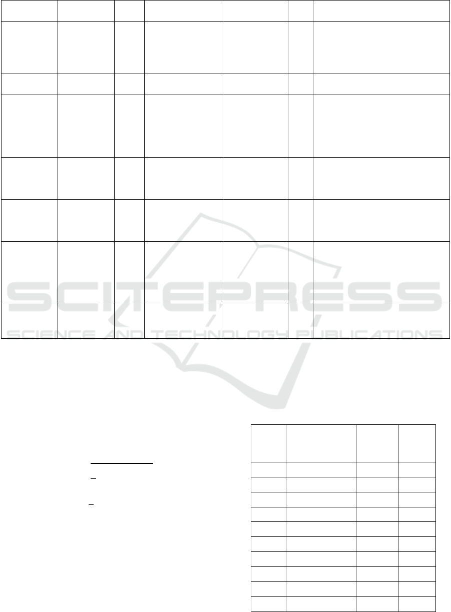
Table 1: Deep learning based BGL prediction: an overview.
Reference Technique Data Architecture
Type of
forecasting
HP
(mn)
Findings
Doike & al.,
2018
Deep
Recurrent NN
CGM
Three hidden layers
with 2000 units,
input and output
layer with one unit
each.
Multi-step-ahea
d
with Direct
strategy
30
A BGL
p
rediction system is used for
hypoglycemia prevention which
achieves an accuracy of 80%.
Mhaskar &
al., 2017
Deep NN CGM 2 layers Not specified 30
The proposed deep NN outperforms
a shallow NN
Xie & Wang,
2018
- LSTM NN
- CNN
CGM
The LSTM NN has
3 hidden LSTM
layers.
The CNN has 2
layers of Temporal
CNN blocks
Multi-step-ahea
d
with Direct and
Recursive
strategy
30
For MSF, AR achieved in average
better performance than LSTM and
CNN.
Direct strategy for LSTM
outperformed the Recursive one.
Fox & al.,
2018
Deep
Recurrent NN
CGM
Two layers with
GRU cells
Multi-step-ahea
d
with MIMO
strategy and
Recursive
30
Multi-output alternatives
outperformed the Recursive ones
El Idrissi &
al., 2019b
LSTM NN CGM
Sequential model:
- One LSTM Layer
- Two fully
connected layers
One-step ahead 5
The proposed LSTM model
significantly outperformed both an
existing LSTM and AR models.
Sun &
al.,2018
LSTM NN CGM
Sequential model:
- One LSTM Layer
- One bidirectional
LSTM layer
- Three fully
connected layers
Multi-step-ahea
d
with Direct
strategy
15, 30,
45, 60
The proposed LSTM outperformed
ARIMA and SVR baseline methods
Mirshekarian
& al., 2017
LSTM NN CGM 5 units LSTM Layer
Multi-step-ahea
d
with Direct
strategy
30, 60
The proposed LSTM NN behaved
similar to an SVR model, and
outperformed physician predictions.
4.2 Performance Criteria
We use two commonly used performance metrics:
root-mean-square error (RMSE) and mean absolute
error (MAE) (El Idrissi & al., 2019a). Let
be the
actual value,
the predicted value, and n the size of
the sample. Equations (6) and (7) present the formula
to calculate the RMSE and MAE respectively.
1
²
(6)
1
|
|
(7)
RMSE and MAE values range in [0,+∞[ , and
higher performance is obtained when RMSE or MAE
tend towards 0.
4.3 Experimental Process
This section describes the experimental process
followed in the empirical evaluation, which consists
of the 3 steps: 1) Data preparation, 2) Performance
evaluation, and 3) Significance tests.
Table 2: Ten patients’ information (El Idrissi & al., 2019b).
The unit of BGL is mg/dl.
Patient
Number of
Recorded BGL
values
Min
BGL
value
Max
BGL
value
P1 766 40 339
P2
278 57 283
P3
283 103 322
P4
923 40 400
P5
562 50 270
P6 771 62 400
P7 897 42 400
P8 546 43 310
P9
831 40 400
P10
246 72 189
HEALTHINF 2020 - 13th International Conference on Health Informatics
340

4.3.1 Step 1: Data Preparation
When training a model, the data should be prepared
to fit the requirements of the model. Thus, given a
time series X = {s(t
i
)} where s(t
i
) is the BGL at time
t
i
, and a sampling horizon d, the time series is
decomposed to couples (X
i
, y
i
), where X
i
={s(t
i-
d+1
),…, s(t
i
)} is the input data and y
i
is the output
value. This decomposition depends on the MSF
strategy we used:
For the Recursive strategy, we have to train a
model that predicts the next value, thus
X
i
={s(t
i-d+1
),…, s(t
i
)} and y
i
=s(t
i+1
).
For the Direct strategy, since the aim is to
predict the BGL value in 30 minutes’ horizon,
we use 6 steps for prediction. Therefore, we
train one model to predict the 6th BGL value.
Thus, the data is presented as X
i
={s(t
i-d+1
),…,
s(t
i
)} and y
i
=s(t
i+6
).
For the MIMO strategy, we have multiple
outputs; therefore, yi is a vector of predicted
BGL values. Hence, a single model is trained
with couples X
i
={s(t
i-d+1
),…, s(t
i
)} and
y
i
={s(t
i+1
),…, s(t
i+6
)}.
For the DirRec strategy, 6 models Ms should
be trained with different sampling horizon. For
each M
s
, the couples are X
i
={s(t
i-d-s+2
),…, s(t
i
)}
and y
i
=s(t
i+1
) where s varies from 1 to 6.
For the DirMO strategy, we set B (i.e. number
of considered blocks) to 2. Therefore, 2 models
are trained: the first model with the couples:
X
i
={s(t
i-d+1
),…, s(t
i
)} and y
i
={s(t
i+1
),…, s(t
i+3
)}
and the second one with X
i
={s(t
i-d+1
),…, s(t
i
)}
and y
i
={s(t
i+4
),…, s(t
i+6
)}.
4.3.2 Step 2: Performance Evaluation
For each strategy, the models are trained and
evaluated for each patient. The dataset of each patient
is divided into training and test data with 66% and
34% of the dataset respectively. The prediction
performance is assessed using RMSE and MAE.
4.3.3 Step 3: Significance Tests
To assess statistically the differences between the
obtained results, we use the Wilcoxon test which is a
non-parametric statistical test. Statistical hypothesis
should be formulated for each hypothesis, and the p-
value is calculated and compared with the
significance level α (Idri & al., 2016a) (Idri & al.
2002) (Idri & al., 2016b).
The statistical tests were done for both criteria
RMSE and MAE two by two, so we obtain 10 Null
Hypothesis (NH) for each criterion: RMSE and
MAE. Each NH is formulated as follow:
NH(I,J,C): There is no difference between the
performances of strategy I and strategy J based on
the criterion C.
All the tests are two-tailed and α is set to 0.05.
The difference will be statistically significant if p-
value is less than α.
To go further in comparison, the sum of ranking
differences (SRD) method was used. This method
proposed by (Héberger, 2010) compares methods or
models based on their ranking. For each model or
method, we sum up the differences between its
ranking and the ideal ranking which corresponds to
the best known method or a reference method. If no
ideal ranking is known, the ideal ranking is obtained
by using the average, the minimum or the maximum
of the all the methods.
5 RESULTS AND DISCUSSION
This section presents and discusses the empirical
results of the five MSF strategies using a LSTM NN
along with the statistical test results. All the empirical
evaluations were carried out using a tool we
developed by Python-3.6 language using the Keras-
2.2.4 framework and Tensorflow-1.12.0 as backend
under Windows 10.
5.1 Results
For each MSF strategy with our LSTM NN, we apply
the steps 1 and 2 of the experimental design in order
to prepare data, train and validate the required
model(s). Each strategy was applied on the 10
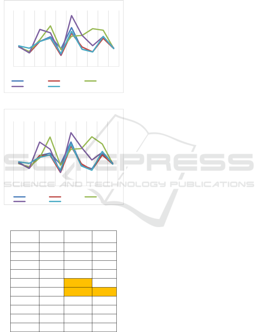
patients of the Figure 1 and Figure 2 present the
RMSE and MAE values of each strategy
respectively.
From Figures Figure
1 and Figure 2, we observe
that the strategies without recursion: Direct, MIMO
and DirMO outperformed in general the strategies
using recursion: Recursive and DirRec. In fact, the
RMSE average for Direct, MIMO and DirMO are
36.30, 34.06 and 35.47 respectively; while the RMSE
average for Recursive and DirRec are 43.76, 42.92
respectively. For the MAE, the average for Direct,
MIMO and DirMO are 28.41, 26.59 and 27.71
respectively; while the MAE average for Recursive
and DirRec are 35.33, 33.42 respectively.
In the third step, the significance tests are
performed using the Wilcoxon statistical test. We
have assessed 20 NHs: 10 NHs for RMSE criterion
and 10 NHs for MAE criterion, and for each one we
Strategies of Multi-Step-ahead Forecasting for Blood Glucose Level using LSTM Neural Networks: A Comparative Study
341
evaluated the p-value. Table 3 presents the p-value
obtained for each NH.
Figure 1: RMSE for the five strategies.
Figure 2: MAE for the five strategies.
Table 3: Results of significance tests.
Strategy 1 Strategy2
p-value for
RMSE
p-value for
MAE
MIMO Direct 0.1141 0.07508
Recursive Direct 0.13888 0.33204
DirRec Direct 0.13888 0.09296
DirMO Direct 0.20408 0.33204
Recursive MIMO 0.03662 0.09296
DirRec MIMO 0.01242 0.01242
DirMO MIMO 0.16758 0.20408
DirRec Recursive 0.71884 0.64552
DirMO Recursive 0.1141 0.20408
DirMO DirRec 0.13888 0.16758
From Table 3, we can conclude that no strategy
outperformed significantly all the others. However,
MIMO significantly outperforms the DirRec strategy
for both RMSE and MAE with p-value equal to
0.01242, and outperforms the Recursive strategy for
RMSE with p-value equal to 0.03662.
5.2 Discussion
The aim of this study was to discuss and answer the
following RQ: What is the MSF strategy that
achieves good performance using the LSTM model
of (El Idrissi & al., 2019b) for an horizon of 30
minutes?. To answer this RQ, five MSF strategies
MSF were used in combination with our LSTM
model using 6-steps ahead, and compared in terms of
RMSE and MAE.
The significance tests performed using Wilcoxon
statistical test did not conclude on the best strategy to
adopt. However, MIMO strategy significantly
outperformed DirRec and Recursive strategies for
RMSE and outperformed DirRec strategy for MAE.
This confirms the trend that we observed from Figure
1 and Figure 2, where we can notice that the
strategies without recursion perform generally better
than those with recursion. This confirms the findings
of the studies (Fox & al., 2018) and (Xie & Wang,
2018): in fact, in (Fox & al., 2018), it was reported
that multi-output alternatives outperformed recursive
ones, and in (Xie & Wang, 2018), the Direct strategy
for LSTM outperformed the Recursive one. This can
be explained by the fact the recursive methods prone
to accumulation errors (Taieb & al., 2012; An & Anh,
2015; Xie & Wang, 2018).
To go further in comparison, we used the SRD
method. In our case, as no ideal ranking is known, we
calculate the ideal ranking based on the minimum
performance all the models. TablesTable
4 andTable
5 show the results of SRD applied on RMSE and
MAE respectively. According to (Héberger, 2010),
the method or model is better when the SRD is
smaller. Thus, using RMSE results, the ranking is:
MIMO, DirMO, Direct, Recursive and DirRec.
Using MAE, we obtain: MIMO, DirMO, Direct,
Recursive, and DirRec.
We conclude that the ranking obtained by SRD
for both RMSE and MAE showed that MIMO is the
best strategy and confirmed the trend that non-
recursive strategies (i.e. MIMO, Direct and DirMO)
are better than recursive ones (i.e. Recursive and
DirRec).
0
10
20
30
40
50
60
70
80
90
P1 P2 P3 P4 P5 P6 P7 P8 P9 P10
Patients
RMSE
Direct MIMO Recursive
DirRec DirMO
0
10
20
30
40
50
60
70
P1 P2 P3 P4 P5 P6 P7 P8 P9 P10
Patients
MAE
Direct MIMO Recursive
DirRec DirMO
HEALTHINF 2020 - 13th International Conference on Health Informatics
342

Table 4: SRD MSF strategies’ ranks for RMSE.
PT. Direct MIMO Rec. DirRec DirMO Min
P1 4 2 0 1 3 1
P2 0 2 3 1 4 1
P3 1 2 3 4 0 1
P4 2 0 4 3 1 1
P5 4 0 3 1 2 1
P6 3 1 0 4 2 1
P7 1 2 3 4 0 1
P8 2 1 4 3 0 1
P9 1 0 4 2 3 1
P10 4 0 2 3 1 1
SRD 22 10 26 26 16 0
Table 5: SRD MSF strategies’ ranks for MAE.
PT. Direct MIMO Rec. DirRec DirMO Min
P1 3 1 0 2 4 1
P2 0 2 3 1 4 1
P3 2 3 0 4 1 1
P4 2 0 4 3 1 1
P5 4 0 3 1 2 1
P6 3 1 0 4 2 1
P7 1 2 3 4 0 1
P8 2 1 4 3 0 1
P9 1 0 4 2 3 1
P10 4 1 2 3 0 1
SRD 22 11 23 27 17 0
6 THREATS TO VALIDITY
We have identified 4 threats to validity for this study:
Internal Validity: it is related to the way the
evaluation was done. To reduce the risk that the
evaluation is not appropriate, 10 datasets were used.
Each dataset was divided on two subsets, training set
used (66%) for training the models and test set (34%)
used for evaluation.
External Validity: the perimeter of the study is
an important threat to take into consideration. To
overcome this issue, we used the dataset of (El Idrissi
& al., 2019b) which contains 10 diabetic patients.
Those patients were randomly taken from a public
dataset and the size of recorded BGL varies from 246
to 923 values.
Construct Validity: this threat is related to the
criteria used to evaluate the MSF strategies’
performance. In this study, the performance was
measured using two criteria which are RMSE and
MAE. Those are common performance measures as
reported by (El Idrissi & al., 2019a).
Statistical Validity: the aim of this study is to
compare the performance of the MSF strategies.
Thus it is important to check if there is a significant
difference between them. For that purpose, the
Wilcoxon statistical test is performed. For ranking,
we used the sum of ranking differences method.
7 CONCLUSIONS AND FUTURE
WORK
A comparative study between five MSF strategies
using a LSTM NN was conducted to assess which
strategies achieved the best performances for BGL
prediction. The five strategies: Recursive, Direct,
MIMO, DirRec and DirMO were used with 6-steps
ahead as the objective is to predict BGL in the next
30 minutes. The performances of the five MSF
strategies were compared in terms of RMSE and
MAE over a 10 patients’ data.
The main findings of the present study were: 1)
no MSF strategy significantly outperformed the
others when using the Wilcoxon statistical test, and
2) MIMO is the best strategy using the Sum of
Ranking Differences method which confirms the
trend that non-recursive strategies are better that
recursive ones.
For future research, we consider carrying out
further empirical evaluations using the five strategies
with other deep learning techniques such as
convolution NNs in order to confirm or refute the
findings of this study.
ACKNOWLEDGEMENTS
This work was conducted within the research project
MPHRPPR1-2016-2020. The authors would like to
thank the Moroccan MESRSFC and CNRST for their
support.
REFERENCES
An, N. H., & Anh, D. T. (2015, November). Comparison
of strategies for multi-step-ahead prediction of time
series using neural network. In 2015 International
Conference on Advanced Computing and Applications
(ACOMP) (pp. 142-149). IEEE.
Bilous, R., Donnelly, R. 2010. Handbook of diabetes. John
Wiley & Sons.
Bontempi, G., Taieb, S. B., & Le Borgne, Y. A. (2012,
July). Machine learning strategies for time series
Strategies of Multi-Step-ahead Forecasting for Blood Glucose Level using LSTM Neural Networks: A Comparative Study
343

forecasting. In European business intelligence summer
school (pp. 62-77). Springer, Berlin, Heidelberg.
DirecNet. (2019). Diabetes Research in Children Network
(DirecNet). Available online at: http://direcnet.jaeb.
org/Studies.aspx [Ap. 1, 2019].
Doike, T., Hayashi, K., Arata, S., Mohammad, K. N.,
Kobayashi, A., & Niitsu, K. (2018, June). A Blood
Glucose Level Prediction System Using Machine
Learning Based on Recurrent Neural Network for
Hypoglycemia Prevention. In 2018 16th IEEE
International New Circuits and Systems Conference
(NEWCAS) (pp. 291-295). IEEE.
El Idrissi, T., Idri, A., & Bakkoury, Z. (2019a). Systematic
map and review of predictive techniques in diabetes
self-management. International Journal of
Information Management, 46, 263-277. https://doi.org/
10.1016/j.ijinfomgt.2018.09.011.
El Idrissi, T., Idri, A., Abnane, I., & Bakkoury, Z. (2019b).
Predicting Blood Glucose using an LSTM Neural
Network. In Proceedings of the 2019 Federated
Conference on Computer Science and Information
Systems. ACSIS, Vol. 18, pages 35–41.
Fox, I., Ang, L., Jaiswal, M., Pop-Busui, R., & Wiens, J.
(2018, July). Deep multi-output forecasting: Learning
to accurately predict blood glucose trajectories. In
Proceedings of the 24th ACM SIGKDD International
Conference on Knowledge Discovery & Data Mining
(pp. 1387-1395). ACM.
Héberger, K. (2010). Sum of ranking differences compares
methods or models fairly. TrAC Trends in Analytical
Chemistry, 29(1), 101-109.
Hochreiter, S., & Schmidhuber, J. (1997). Long short-term
memory. Neural computation, 9(8), 1735-1780.
Idri, A., Abnane, I., & Abran, A. (2016a). Missing data
techniques in analogy-based software development
effort estimation. Journal of Systems and Software,
117, 595-611.
Idri A, Khoshgoftaar TM, Abran A. (2002). Investigating
soft computing in casebased reasoning for software
cost estimation. Eng Intell Syst Elec. 10(3):147-157.
Idri A, Hosni M, Abran A. (2016b). Improved estimation
of software development effort using classical and
fuzzy analogy ensembles. Appl Soft Comput. 49:990-
1019.
Kline, D. M. (2004). Methods for multi-step time series
forecasting neural networks. In Neural networks in
business forecasting (pp. 226-250). IGI Global.
Mhaskar, H. N., Pereverzyev, S. V., & van der Walt, M. D.
(2017). A deep learning approach to diabetic blood
glucose prediction. Frontiers in Applied Mathematics
and Statistics, 3, 14.
Mirshekarian, S., Bunescu, R., Marling, C., & Schwartz, F.
(2017, July). Using LSTMs to learn physiological
models of blood glucose behavior. In 2017 39th Annual
International Conference of the IEEE Engineering in
Medicine and Biology Society (EMBC) (pp. 2887-
2891). IEEE.
Sorjamaa, A., & Lendasse, A. (2006, April). Time series
prediction using DirRec strategy. In
Esann (Vol. 6, pp.
143-148).
Sorjamaa, A., Hao, J., Reyhani, N., Ji, Y., & Lendasse, A.
(2007). Methodology for long-term prediction of time
series. Neurocomputing, 70(16-18), 2861-2869.
Sun, Q., Jankovic, M. V., Bally, L., & Mougiakakou, S. G.
(2018, November). Predicting Blood Glucose with an
LSTM and Bi-LSTM Based Deep Neural Network. In
2018 14th Symposium on Neural Networks and
Applications (NEUREL) (pp. 1-5). IEEE.
Taieb, S. B., Bontempi, G., Atiya, A. F., & Sorjamaa, A.
(2012). A review and comparison of strategies for
multi-step ahead time series forecasting based on the
NN5 forecasting competition. Expert systems with
applications, 39(8), 7067-7083.
Taieb, S. B., Bontempi, G., Sorjamaa, A., & Lendasse, A.
(2009, June). Long-term prediction of time series by
combining direct and mimo strategies. In 2009
International Joint Conference on Neural Networks
(pp. 3054-3061). IEEE.
Xie, J., & Wang, Q. (2018, January). Benchmark Machine
Learning Approaches with Classical Time Series
Approaches on the Blood Glucose Level Prediction
Challenge. In KHD@ IJCAI (pp. 97-102).
HEALTHINF 2020 - 13th International Conference on Health Informatics
344
