Predicting Location Probabilities of Drivers to Improve

Dispatch Decisions of Transportation Network Companies

based on Trajectory Data

Keven Richly, Janos Brauer and Rainer Schlosser

Hasso Plattner Institute, University of Potsdam, Potsdam, Germany

Keywords:

Trajectory Data, Location Prediction Algorithm, Peer-to-Peer Ridesharing, Transport Network Companies,

Risk-aware Dispatching.

Abstract:

The demand for peer-to-peer ridesharing services increased over the last years rapidly. To cost-efﬁciently

dispatch orders and communicate accurate pick-up times is challenging as the current location of each avail-

able driver is not exactly known since observed locations can be outdated for several seconds. The developed

trajectory visualization tool enables transportation network companies to analyze dispatch processes and de-

termine the causes of unexpected delays. As dispatching algorithms are based on the accuracy of arrival time

predictions, we account for factors like noise, sample rate, technical and economic limitations as well as the

duration of the entire process as they have an impact on the accuracy of spatio-temporal data. To improve

dispatching strategies, we propose a prediction approach that provides a probability distribution for a driver’s

future locations based on patterns observed in past trajectories. We demonstrate the capabilities of our predic-

tion results to (i) avoid critical delays, (ii) to estimate waiting times with higher conﬁdence, and (iii) to enable

risk considerations in dispatching strategies.

1 INTRODUCTION

The usage of transport network companies (e.g., Ca-

reem, Lyft, or Uber) rapidly increased over the last

years. These companies offer a peer-to-peer rideshar-

ing service by connecting vehicle drivers with pas-

sengers to provide ﬂexible and on-demand transporta-

tion (Masoud and Jayakrishnan, 2017). Based on in-

coming passenger requests, the ride-hailing service

provider has to assign an order (request) to an appro-

priate driver from a pool of available drivers, which

are constantly moving in a road network freely. For

that reason, it is necessary to have exact location in-

formation of all drivers to i) optimize the order dis-

patching process and ii) communicate accurate wait-

ing times to passengers.

The dispatching of orders focuses on reducing the

overall travel time and waiting time of passengers, op-

timizing the utilization of available resources, and in-

creasing the customer expectations (Xu et al., 2018).

There is a wide spectrum of dispatching algorithms

that determine the potential best candidate for an or-

der on the basis of various aspects. Spatio-temporal

cost functions, which are calculated based on the cur-

rent location of drivers and passengers, are an integral

part of these algorithms (Liao, 2003). Examples for

such metrics are the distance to the pick-up location

or the estimated time to reach the pick-up location.

Due to the evaluation of trajectory data of avail-

able drivers, a detailed analysis of dispatch decisions

is possible. It enables transportation network com-

panies to identify limitations of dispatching policies

and allows the comparison of different strategies and

conﬁgurations. By inspecting the dispatching process

of bookings, the causes for unexpected critical delays

can be investigated and an understanding of poten-

tially risky scenarios can be developed.

As one cause for delayed pick-up times and sub-

optimal dispatch decisions, we identiﬁed the inaccu-

racy and uncertainty of the driver’s exact location,

which is used for the travel time estimation and the or-

der dispatching. Surrounding urban effects cause sig-

nals to be noisy and lead to deviations of the recorded

GPS location and the real one of a driver (Wang

et al., 2011). Additionally, the technical limitations

of the GPS system and economical considerations

constrain the emission of signals. To reduce band-

width and storage costs, drivers’ GPS locations are

recorded and sent in speciﬁc intervals respecting a de-

ﬁned sampling rate. Furthermore, the entire dispatch

Richly, K., Brauer, J. and Schlosser, R.

Predicting Location Probabilities of Drivers to Improve Dispatch Decisions of Transportation Network Companies based on Trajectory Data.

DOI: 10.5220/0008911100470058

In Proceedings of the 9th International Conference on Operations Research and Enterprise Systems (ICORES 2020), pages 47-58

ISBN: 978-989-758-396-4; ISSN: 2184-4372

process, including the acceptance conﬁrmation by the

driver, consumes several seconds, in which the driver

is changing the position.

Based on these observations, it is necessary to an-

alyze and optimize the used locations of drives to im-

prove the accuracy of arrival time predictions and op-

timize order dispatch algorithms.

The contributions in this work are the following:

• We implemented a trajectory visualization tool,

which enables transportation network companies

to analyze their dispatch processes and determine

the causes of unexpected critical delays.

• We propose a location prediction approach, which

determines a distribution of potential future loca-

tions of drivers based on patterns observed in past

trajectories.

• Compared to common dispatching algorithms that

rely on outdated driver positions only, we are

able to avoid critical delays by assigning drivers

based on their estimated current potential position

accounting for their individual driving behavior

(speed, turn probabilities, etc.).

• We demonstrate that the prediction results allow

to forecast potential waiting times with higher

conﬁdence which, in turn, effectively helps to de-

crease customers’ cancellation rates.

This paper is organized as follows. In Section 2

we describe the problem domain. Afterward, we

present the developed application to analyze dispatch

processes (Section 3). In Section 4, we present the

limitations of dispatch decisions based on the last

observed location of drivers. In Section 5, we de-

scribe our probabilistic location prediction approach.

In Section 6, we present related work. Conclusions

are given in the last section.

2 BACKGROUND

In the following section, we deﬁne all relevant infor-

mation entities that are part of the problem domain

and necessary to understand the visualization con-

cepts as well as the proposed algorithm to avoid risky

dispatches.

A road network is a directed multigraph that rep-

resents real-world trafﬁc infrastructure of a spec-

iﬁed area along with the corresponding meta-

data (Ben Ticha et al., 2018). In the graph, each

node represents an intersection between at least two

road segments, which are represented by edges.

These road network maps are created and maintained

by humans or automatically updated by trajectory-

based algorithms (He et al., 2018). The meta-

information includes, for example, the length and

speed limit of a road segment as well as the exact ge-

ographic locations for all intersections and road seg-

ments (Ben Ticha et al., 2018).

Deﬁnition 2.1. Road Network: A road network

is a multigraph R represented by a 4-tuple R =

(I, E, Σ

, Σ

). I is a set of nodes representing inter-

sections. Σ

and Σ

contain the node and edge la-

bels, respectively. E ⊆ V × V × Σ

is the set of edges

encoding road segments between intersections. The

node labels Σ

are composed of an intersection’s GPS

location, whereas the edge labels Σ

consist of a road

segment’s geographic extent, length, and speed limit.

Deﬁnition 2.2. Road Segment: A road segment r is a

directed edge that is conﬁned by a source r.source and

target r.target intersection. It is associated with a list

of intermediate GPS points describing the segment’s

geography. Each road segment contains a length and

a speed limit. A set of connecting road segment com-

poses a road.

In this work, a trajectory is a chronologically or-

dered sequence of map-matched and timestamped ob-

served locations of a driver, which represents a con-

tinuous driving session. For that reason, we use a seg-

mentation algorithm to split the raw positional data of

a single moving object into separate trajectories. The

start and end of driving sessions are deﬁned by events

like changes of the occupancy state or inactive time

intervals of drivers.

Deﬁnition 2.3. Trajectory: A trajectory T

is a

chronologically ordered sequence of map-matched

and timestamped observed locations of a driver d in

a given time interval [t

, t

Deﬁnition 2.4. Ping: A ping p

depicts a map-

matched observed location of a driver d at time t. The

state p

is given by a 3-tuple (l, s, t), denoting that the

driver d is located at location l with the occupancy

state s at time t. The location l consists of the tuple

(x, y) representing the map-matched GPS coordinates

with longitude and latitude.

As mentioned in the previous section, the accu-

racy of GPS locations is affected by various factors

(e.g., noise) (Wang et al., 2011). For that reason, it

is possible that the observed locations of a driver are

off-road. Therefore, we use common map-matching

algorithms to match the locations to a reference road

network. For each observed location a map-matched

location on a road segment is determined based on the

trajectory of a driver.

ICORES 2020 - 9th International Conference on Operations Research and Enterprise Systems

3 VISUALIZATION OF DISPATCH

PROCESSES

With the capabilities to display the trajectory data, our

application enables transportation network companies

(i) to analyze dispatch decisions, (ii) to evaluate and

compare different dispatching algorithms, (iii) to de-

termine the effect and accuracy of location predic-

tion algorithms, and (iv) to label spatio-temporal data

for comprehensive investigations or as foundation for

machine learning approaches. Through the detailed

analysis of past dispatches, it is possible to identify

reasons for late pick-ups and determine characteris-

tics of scenarios, in which the risk for a delay exists.

Additionally, it provides the opportunity to identify

general problems of dispatch strategies and to exam-

ine the behavior in edge cases.

3.1 Analyzing Dispatch Decisions

An overview of bookings enables transportation net-

work companies to navigate through various dis-

patch processes to identify problematic dispatches ef-

ﬁciently (e.g., signiﬁcant delays). The bookings can

be ﬁltered and sorted by different criteria (e.g., delay,

manually assigned labels) to select speciﬁc dispatches

to be analyzed in more detail (see Figure 1).

In the analysis view, the system visualizes the

spatio-temporal data associated with the dispatch de-

cision on a map. As shown in Figure 1, the trajec-

tory of the assigned driver (colored dots), the posi-

tion of the pick-up location (black marker), and the

shortest route to the pick-up location (green line) are

displayed. Additionally, the corresponding informa-

tion (e.g., estimated time of arrival determined by the

transportation network company and the Open Source

Routing Machine (OSRM)

) are shown. The tra-

jectory of the driver is divided into orange and blue

dots, which represent the associated pings. The color

change indicates the timestamp at which the driver

acknowledged the transportation request, and the trip

was assigned. Consequently, the orange points repre-

sent the free-time trajectory of the driver. In periods

without passengers or passenger requests, the drivers

drive freely around intending to get in an excellent po-

sition to be selected by the dispatch algorithm for the

next booking request.

The blue dots of the trajectory represent the route

of the driver after the assignment of the trip. Here,

the driver has a particular target location and tries to

reach the pick-up location on the shortest path. By

comparing this trajectory with the shortest path de-

termined by OSRM, the user has a good indicator of

http://project-osrm.org

problematic dispatches. As displayed in the exam-

ple (see Figure 1), the delay of the driver was caused

by an initial detour. Furthermore, we can analyze the

circumstances around the assignment of the trip and

determine potential reasons for the detour (e.g., inac-

curate positional information or a driver’s position on

a road segment, which makes it impossible for him

to drive the shortest route). In Section 4, we discuss

these issues in more detail.

To evaluate different prediction algorithms as

well as our probabilistic approach (described in Sec-

tion 5), the application visualizes the predicted loca-

tions along with the determined probabilities. The lo-

cations are displayed directly on the map to allow the

user to compare the predicted positions (purple cir-

cles) with the last observed location and the trajectory

of the driver after the dispatch process.

3.2 Determining the Estimated Fastest

Pickup Routes

The application illustrates the fastest route between

the last ping of the dispatched driver’s free-time tra-

jectory and pick-up location as a solid line. We use

the OSRM, a tool of the OpenStreetMap community,

to calculate a driver’s fastest pick-up route. In con-

trast to routing services used by deployed dispatching

algorithms of transportation network companies, the

routing functionality of OSRM is not trafﬁc-adjusted.

Instead, it estimates the cost of a road segment, i.e.,

its traversal time, as its length divided by its speed

limit. The traversal speed estimation via the speed

limit is a signiﬁcant simpliﬁcation, as the scenario that

a driver traverses the road network without any trafﬁc

and with traversal speed indicated by the speed limit

is very unlikely.

However, this constraint is acceptable, as even if

we use the same trafﬁc-adjusted routing service as the

deployed dispatching algorithm, the calculated pick-

up route and its traversal time may differ from the

route the dispatching algorithm has retrieved at the

time of the dispatch from the same service. The rea-

son is that routing services, such as Google Maps,

incorporate trafﬁc in real-time to keep estimates ac-

curate and hence, the suggested fastest route for the

same pair of GPS coordinates changes continuously

with the underlying trafﬁc. The fastest pick-up route

that we retrieve from OSRM is not guaranteed to be

identical to the pick-up route that was used by the

dispatching algorithm. Hence, the estimated traver-

sal time of the fastest pick-up route and the estimated

traversal time calculated by the dispatching algorithm

of the transportation network company are not com-

parable to each other.

Predicting Location Probabilities of Drivers to Improve Dispatch Decisions of Transportation Network Companies based on Trajectory Data

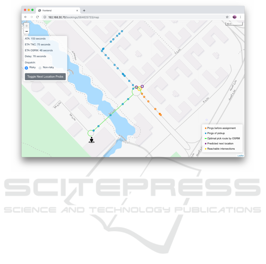
Figure 1: A screenshot of the application, displaying the trajectory of the driver (orange and blue dots), the fastest route (green

line), and the predicted next locations via purple circles.

4 IMPROVING DISPATCH

DECISION BY LOCATION

PREDICTION ALGORITHMS

As already mentioned, it is necessary to provide exact

location information of all available drivers to com-

municate accurate pick-up times to passengers and to

efﬁciently assign passengers to drivers. The assign-

ment of available drivers to requesting passengers in

the context of transportation network companies is a

dynamic vehicle routing problem or dial a ride prob-

lem.

The vehicle routing problem is characterized as

dynamic, if requests are received and updated concur-

rently with the determination of routes, see Psaraftis

et al. (Psaraftis, 1995). In the setup of transporta-

tion network companies, new passenger requests have

to be continuously assigned to available drivers con-

sidering further information, such as the current traf-

ﬁc situation or the availability of drivers, which are

unknown in advance. For that reason, companies

are applying different policies typically intending to

optimize speciﬁc objective functions (e.g., to mini-

mize the overall waiting time of passengers or route

costs) (Psaraftis et al., 2016).

Correspondingly, the applied policy to select a

driver from a set of available drivers is based on a cost

function (e.g., minimum costs, minimum distance,

minimum travel time, maximum number of passen-

gers). Most of these functions use the location of the

passengers and the location of the available drivers

as inputs. A common example is the nearest vehicle

dispatch, which assigns the passenger request to the

driver with the shortest travel time to the pick-up lo-

cation (Jung et al., 2013). Based on the locations, the

travel time is determined by using services that offer

trafﬁc-adjusted routing services (e.g., Google Maps).

For that reason, accurate calculations require pre-

cise and up-to-date location information about all

available drivers. However, there are different fac-

tors like noise or technical limitations of GPS sys-

tem (Wang et al., 2011).

Additionally, the given sampling rate, data trans-

fer problems, and the time consumed by the entire

process affects the accuracy of the spatio-temporal

information. Consequently, the actual position of a

driver at the time of the order assignment can deviate

signiﬁcantly from the last observed location, which

is currently used as input to calculate the estimated

travel time or distance.

ICORES 2020 - 9th International Conference on Operations Research and Enterprise Systems

Figure 2: An example highlighting the implications of the

driver’s current location’s inaccuracy and uncertainty. The

dotted location marker between the two highway lanes de-

picts the last recorded location. The other markers indicate

a driver’s possible current locations on the two roads.

4.1 Limitations of Status - Quo

Dispatch Decisions

To demonstrate the limitations of dispatch decisions

based on the last observed location, we use the dis-

patching example depicted in Figure 2 to exemplify

the implications of the inaccuracy and uncertainty of

a driver’s current location at the time of dispatch. The

example shows a dispatching scenario on a highway,

where the upper-right user pin represents the passen-

ger’s pick-up location and the car pins represent a sin-

gle driver’s GPS locations. While the dotted marker

represents the driver’s last recorded location (which

the dispatching algorithm uses), the solid markers

represent the driver’s possible locations at the time of

dispatch. The driver’s last recorded position in the ex-

ample is affected by noise so that the recorded loca-

tion resides between the two highway lanes. Depend-

ing on its implementation, the dispatching algorithm

may now assume that the driver is on the right lane,

however, if the driver’s correct location is A, the ac-

tual travel time can be much higher than its estimated

counterpart, as turns on highways are impossible and

the next exit may be far away.

Even when on the right side of the street, the

driver’s location at the time of dispatch relative to the

necessary highway exit is unknown: the driver may

have or may not have taken the exit (location D and

C), or the driver may not have reached the exit (lo-

cation B). The actual travel time varies signiﬁcantly

with locations B − D, as missed exists on highways

are costly in terms of time. Consequently, there is

a high risk of delay. Additionally, the driver’s last

recorded location may be older than indicated by the

sampling rate or urban effects, such as tunnels, pre-

vent the emission of GPS signals. Also, the entire

process of assigning a driver and the acknowledgment

of the drive takes several seconds, where the position

of the driver is continuously changing.

As shown by the example, an inaccuracy and un-

certainty of the drivers’ locations at the time of dis-

patch can signiﬁcantly inﬂuence the determined value

of the cost function (e.g., travel time). Therefore, the

dispatching algorithm has to decide based on incor-

rect information, for which reason it may not assign

the optimal driver to a requesting passenger and also

the driver could arrive delayed at the pick-up location.

For that reason, we introduce the concept of Detoured

Dispatches and Risky Dispatches, see below.

Deﬁnition 4.1. Detoured Dispatch: A dispatch is

classiﬁed as a detoured dispatch if the assigned

driver’s arrival at the pick-up location is delayed due

to an initial detour of the driver.

Deﬁnition 4.2. Risky Dispatch: A dispatch is said to

be risky if the dispatched driver’s arrival at the pick-

up location is likely to be delayed due to uncertainty

about the current position of a driver, which may lead

to an initial detour or a sub-optimal route.

After the selection of a driver, the exact current

position is also necessary to calculate the estimated

waiting time, which is communicated to the customer.

The waiting time has to be accurate as the cancella-

tion rate strongly increases with the displayed wait-

ing time. High cancellation rates reﬂect unsatisﬁed

passengers leading to a drop in passenger retention

rate, as the industry of ride-hailing is characterized

by ﬁerce competition. Ultimately, high cancellation

rates reduce the revenue of a transportation network

company. The communicated waiting time has to be

accurate, i.e., the actual travel time cannot be much

longer than the calculated travel time. Otherwise, the

passenger has to wait longer than initially communi-

cated, leading to an increase in the cancellation rate.

We observed that passengers do not tolerate delays,

as more than 50% of all delay-related cancellations

happen within the ﬁrst two minutes of a delay.

To evaluate the share of delays caused by detoured

dispatches, we analyzed a sample of 500 dispatch de-

cisions with our application manually. The dispatch

processes were randomly selected from a real-world

dataset of a transportation network company, which

includes the bookings and the spatio-temporal data

of Dubai, spanning from November 2018 to February

2019. Further, we limited the analysis to dispatch pro-

cesses where the driver arrived at the pick-up location

between one and ﬁve minutes delayed. We classiﬁed a

dispatch as detoured if the driver performed an initial

detour after the conﬁrmation of the trip and returned

Predicting Location Probabilities of Drivers to Improve Dispatch Decisions of Transportation Network Companies based on Trajectory Data

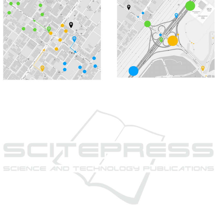
Figure 3: Predicting potential current locations of candi-

date drivers to be assigned to a waiting customer (black

marker): Example of three different drivers (green, blue,

orange marker). The dots represent predicted potential next

locations of each driver based on their driving behavior.

to the determined fastest route afterward. Based on

the random sample, we identiﬁed that in about 20 per-

cent of the delayed arrivals, the driver performed an

initial detour.

4.2 Probabilistic Location Predictions

and Implications for Dispatch

Decisions

An example of how probabilistic location predication

can inﬂuence the dispatch decisions is shown in Fig-

ure 3. The black marker represents the pick-up lo-

cation and the blue, green, and orange markers the

last observed map-matched location of three avail-

able drivers. A traditional dispatching algorithm that

uses a speciﬁc cost function (e.g., shortest distance or

shortest travel time) would assign the booking request

to the blue driver based on the last observed locations.

By analyzing the predicted potential positions of the

drivers, we can see that the blue and green drivers are

likely to move away from the location of the passen-

ger. In contrast, the orange driver is directly driving

in the direction of the passenger. For that reason, it is

highly likely that the orange driver would be the best

option for the algorithm.

In this example, we demonstrate that by includ-

ing the driving behavior and direction of drivers, the

result of the dispatch algorithm can change. Addition-

ally, we can immediately detect whether the estimated

time of arrival of a certain driver (e.g., the blue driver

in Figure 4) would be too optimistic and detours and,

in turn, critical delays are likely.

In the second example (see Figure 4), we demon-

Figure 4: Improving dispatch decisions using probability

distributions for the current locations of potential drivers:

Comparing the likelihood of a driver to reach the customer

(black marker) without critical delays. Example of three

different drivers (green, blue, orange marker). The dots rep-

resent the predicted next locations of each driver (the larger

the dot is, the higher is the probability of the location).

strate the impact of the probabilities calculated based

on observed patterns in past drives. The size of the

dots represents the probability of the corresponding

location. The larger a dot is, the higher is the proba-

bility of the location. Similar to the ﬁrst example (see

Figure 4), the blue driver has the shortest distance and

seemingly the shortest travel time to the pick-up loca-

tion. But the big dot in the left-bottom corner indi-

cates that there is a high chance that the blue driver

misses the exit. For that reason, it may be preferable

to assign the trip to another driver.

The green driver has a higher probability of be-

ing on the shortest route to the pick-up location, but

also there is a not negligible probability that the driver

stays on the highway and needs to perform a costly

detour to reach the location of the passenger.

Based on the last observed location, the orange

driver has the longest distance to the pick-up loca-

tion, but the predicted probabilities show that she is

highly likely driving the direction of the pick-up loca-

tion. Consequently, to assign the order to the orange

driver is potentially not the optimal decision, but the

one with the lower risk of delays.

Our proposed approach enables transportation

network companies to apply dispatching strategies

that take risk considerations into account. Whether to

optimize expected arrival times, worst-case scenarios,

or other risk-aware criteria can be strategically deter-

mined by the companies. Our approach, however, is a

key for such risk-aware dispatching strategies.

ICORES 2020 - 9th International Conference on Operations Research and Enterprise Systems

5 PROBABILISTIC LOCATION

PREDICTION FOR

RISK-AWARE DISPATCHING

To minimize detoured dispatches and enable risk-

aware decisions, we propose a model to predict prob-

abilities of future driver positions based on patterns

observed in past trajectories. We suggest the algo-

rithm to be used to predict the possible locations of

dispatching candidates at the time of assignment of

the trip. The dispatching algorithm calculates the es-

timated travel time from a combination of travel times

considering the set of possible locations. By min-

ing historic drives and predicting possible locations

allows for a more precise estimation of pick-up times

leading to shorter waits, in spite of the inherent uncer-

tainty and inaccuracy of a driver’s current position.

5.1 Description of the Probabilistic

Location Prediction Algorithm

The goal of this approach is to observe repeating driv-

ing patterns from all drivers that can be generalized so

that we can apply them to forecast upcoming driving

behaviors. The generalization requires the analysis

of past driving behavior that is representative of fu-

ture behavior. As we forecast a driver’s next locations

around the time of dispatch, we constrain the analysis’

dataset to free-time trajectories. In free-time trajecto-

ries, drivers are generally not inﬂuenced by external

factors and thus can drive freely around.

At the time of dispatch, drivers are unaware of a

request until it is communicated to them, which is af-

ter the dispatch process. Consequently, at the time of

dispatch drivers drive freely around, and hence, their

decisions are similar to the ones taken before in past

free-time trajectories. The analysis of trajectories also

allows us to extract information on the dynamic char-

acteristics of the road network, such as trafﬁc. Traf-

ﬁc affects drivers’ traversal times on road segments

and hence we need to incorporate this into the loca-

tion prediction to ensure accuracy. Trafﬁc repeats it-

self (Treiber and Kesting, 2013), we can use histori-

cal trafﬁc patterns to forecast future traversal times on

road segments consequently.

Remark 5.1. The prediction algorithm consists of the

ﬁve parts (i) data preprocessing, (ii) map matching,

(iii) road segment candidates determination, (iv) turn

probability calculation, and (v) location prediction.

Most importantly, the ﬁnal prediction of a driver’s

probabilistic location takes not more than 30 millisec-

onds, and hence, is applicable in real-life settings.

Note, part (i), (ii), and (iv) of the algorithm can be

processed ofﬂine and updated from time to time.

5.1.1 Data Preprocessing

During the data preprocessing, we segment the trajec-

tories in sub-trajectories that represent distinct driv-

ing sessions and extract the sub-trajectories with the

occupancy state free. Afterward, we map-match the

observed locations to retrieve their actual location on

a road segment in the road network. Based on the

map-matched pings, we interpolate the route between

subsequent pings if their road segments are discon-

tiguous.

Depending on the occupancy state, the driving be-

havior of a driver changes signiﬁcantly. If the driver

is transporting passengers or is on the way to pick-up

passengers, she is driving the shortest route based on

the current position, the destination, and the current

trafﬁc situation. These routes are often suggested by

routing services.

In contrast, drivers with the occupancy state free

are freely driving around with the goal of getting in-

coming bookings. Their routes are depending on per-

sonal experience and individual preferences as well

as external circumstances. For that reason, we have to

distinguish trajectories based on the occupancy state

for our use case.

Deﬁnition 5.1. Occupancy State of Trajectory: The

occupancy state of a trajectory T

is deﬁned by the

state of all pings of the trajectory. For that reason, all

pings of a trajectory must have the same occupancy

state. We distinguish between the two states available

and occupied.

We deﬁne a route as an ordered sequence of con-

nected road segments, which are determined by the

trajectory and deﬁnes a semantic compression of the

trajectory consequently. Multiple consecutive pings

on a road segment are combined. Additionally, if the

resulting road segments are not connected, the corre-

sponding road segments to connect the segments by

the shortest path are added to the route.

Deﬁnition 5.2. Route: A route R

of a driver d

is a sequence of connected road segments, visited by

driver d in the time interval [t

, t

] ordered by the time

of traversal.

A booking represents a transportation request

from a passenger. During dispatch, a potential driver

is assigned to the booking. After the driver conﬁrms

the booking, her occupancy state changes from avail-

able to occupied. Accordingly, the state changes to

available after the driver ﬁnished a booking.

Predicting Location Probabilities of Drivers to Improve Dispatch Decisions of Transportation Network Companies based on Trajectory Data

5.1.2 Map Matching

The accuracy of GPS locations is affected by var-

ious factors (e.g., noise) (Wang et al., 2011), cf.

Section 2. To match the locations to a reference

road network, we use the established map-matching

library Barefoot

. Additionally, we applied ﬁlters

to remove physically implausible sequences of map-

matched location caused by the breaks in the Hidden

Markov Model used by this approach. Newson and

Krumm (Newson and Krumm, 2009), also suggest ﬁl-

ter and cleansing approaches for outliers (e.g., traver-

sal speed and maximum acceleration thresholds).

5.1.3 Road Segment Candidates

To determine the relevant potential road segments on

which the driver is estimated to be after the predic-

tion frame based on the last observed location, we

partially analyze the road network. Each road seg-

ment has an associated cost, which depicts its traver-

sal time (i.e., the time a driver needs to traverse it

completely). There are different approaches to de-

termine the traversal time (e.g., speed limits, actual

speed of the driver). We use an approach that mines

the traversal speed from past trajectories.

The mined traversal speed is the average speed of

all drivers on the road segment of past trajectories

(e.g., of a given hour). Due to the fact that we con-

sider all pings of a driver on a speciﬁc road segment,

the mined traversal speed implicitly includes trafﬁc

effects like trafﬁc light phases or trafﬁc jams. Start-

ing from the road segment of the last ping, we de-

termine all possible paths of the driver by summing

up the traversal times of the road segments until the

prediction frame is exceeded. By deﬁnition, the algo-

rithm expects drivers to reach the last road segment of

a path and we add the last road segment to the list of

candidates consequently. Instead of considering just

all road segments in the neighbourhood, this approach

allows to derive a set of road segments that includes

all potential ones and is as small as possible, which in

turn allows for faster predictions.

5.1.4 Calculation of Turn Probabilities

To determine the turning behavior at intersections,

we can count the co-occurrences of road segment

pairs (Krumm, 2016; Liu and Karimi, 2006) and cal-

culated the corresponding probabilities. We model

the turn probabilities by a Markov chain of n

-order,

as a driver’s behavior at intersections can be repre-

sented by a sequence of events, in which the proba-

https://github.com/bmwcarit/barefoot

bility of each event, i.e., the decision at the current

intersection, depends only on the state attained in the

previous event, i.e., the decision at the previous inter-

section. Markov chains of a higher order allow us to

represent the behavior of drivers better to drive around

a speciﬁc area. This behavior is not uncommon for

drivers of transportation network companies, due to

the fact that speciﬁc regions are more proﬁtable com-

pared to others (Richly and Teusner, 2016).

5.1.5 Final Location Prediction

At the last step, we extrapolate a driver’s speciﬁc lo-

cation on the determined road segments, as the esti-

mated time to the passenger can vary based on the

particular location on a road segment. During the

short-term route prediction, we calculate a set of road

segments candidates that a driver is expected to reach

within the prediction frame f . We determine for each

candidate road segment a driver’s required traver-

sal time t

path

∈ R

to reach it. As the remaining

time t

remaining

of each candidate road segment, i.e.,

remaining

= f − t

path

, is not large enough to traverse it

completely, we expected the driver to be located on it.

Given each candidates remaining and traversal time,

we estimate the drivers detailed position via the frac-

tion of the road segment the driver is expected to have

traversed within the prediction frame.

5.2 Numerical Evaluation

In this section, we evaluate the accuracy of our loca-

tion prediction algorithm. We perform out-of-sample

four-fold cross-validation for all experiments and re-

port the average score over all four runs.

5.2.1 Experimental Setup

To evaluate our approach, we used a real-world tra-

jectory dataset of a renowned transportation network

company. The dataset includes observed locations of

drivers and booking information in the city of Dubai,

spanning from November 2018 to February 2019.

Compared to publicly available datasets, it has a high

sampling rate of 5 seconds. For the period, we have

over 400 million observed locations.

Based on the time span between two observed lo-

cations, we segment the trajectory data of a driver in

sub-trajectories representing continuous driving ses-

sion. We classiﬁed the sub-trajectories based on the

occupancy state and get 1.5 million free-time trajec-

tories. The OpenStreetMap road network of Dubai

has 139K road segments with average length of 115m.

ICORES 2020 - 9th International Conference on Operations Research and Enterprise Systems

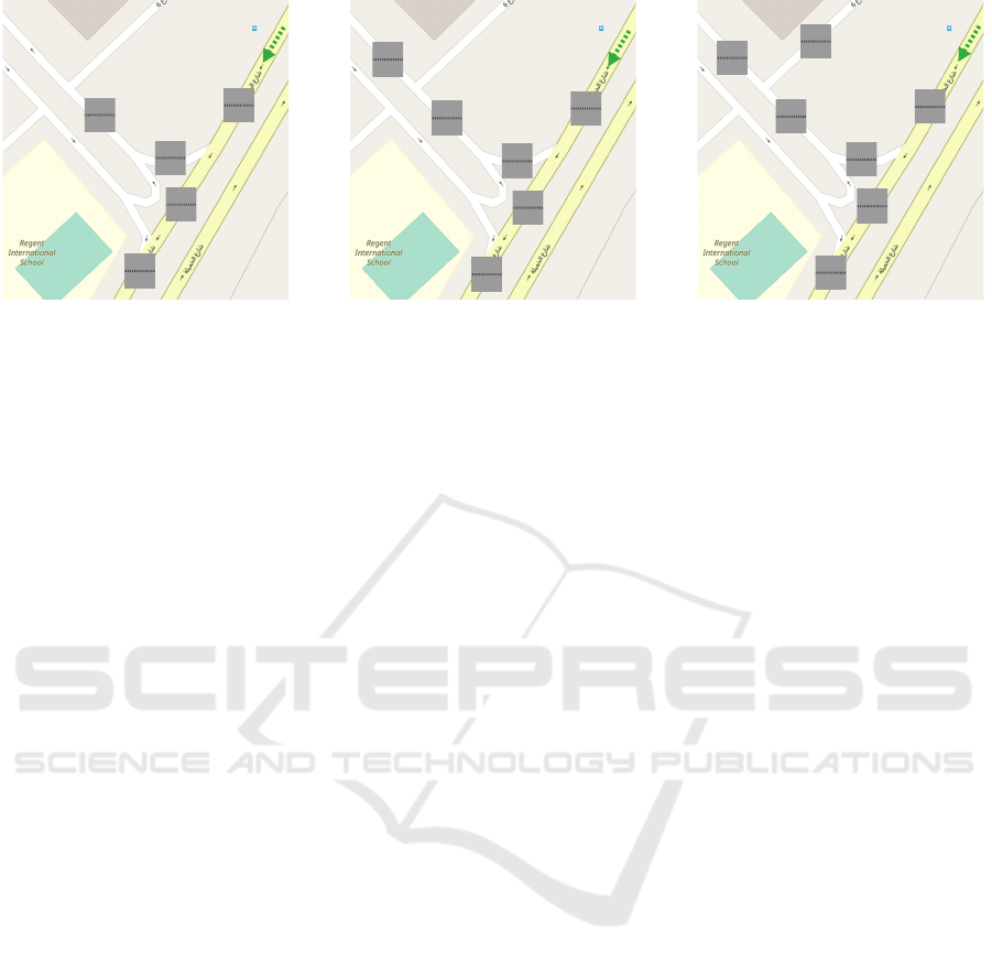
0.007

0.001

0.245

0.239

0.504

0.501

0.196

0.227

0.048

0.032

(a) prediction frame: 5 s

0.114

0.085

0.004

0.000

0.130

0.172

0.508

0.458

0.106

0.164

0.138

0.121

(b) prediction frame: 10 s

0.102

0.227

0.003

0.001

0.131

0.018

0.042

0.065

0.500

0.352

0.018

0.058

0.204

0.280

Figure 5: Results of the next location prediction algorithm on a representative road segment. We run the experiment on 1 000

out-of-sample pings that share the same road segment indicated by the dashed green arrow. The upper value in the box denotes

the relative frequency of drivers that are on the respective road segment after the prediction frame. In contrast, the value below

depicts the probability we predict for drivers to be on that road segment after the prediction frame.

5.2.2 Evaluation of the Prediction Algorithm

We evaluate the overall quality of the next location

prediction algorithm. We use 1 000 pings located on

the same road segment, to predict the road segments

their associated drivers could be on after the predic-

tion frame, i.e., the road segment candidates, along

with their respective probabilities. The drivers’ cor-

rect road segment after the prediction frame serves as

the ground truth.

We compare the discrete probability distribution

of these predicted road segments with the discrete

relative frequency distribution of the drivers’ correct

road segments of the ground truth. We model the turn-

ing behavior via 2

-order Markov chains. For the ex-

periments, we set the prediction frame to 5, 10, and 20

seconds and evaluate the algorithm’s performance for

a representative example.

In Figure 5, we illustrate the results of our loca-

tion prediction algorithm for drivers that are currently

on a frequented road segment. The training dataset

for the algorithm includes 21 751 traversal speed ob-

servations and 9 224 turn observations for the respec-

tive road segments. The predicted probability density

over the set of road segment candidates is similar to

the distribution of the relative frequencies of the in-

dividual road segments of the ground truth. The av-

erage absolute difference between the probability of

a predicted road segment and its relative frequency in

the ground truth for the prediction frames are small:

0.012 (5 seconds), 0.033 (10 seconds), and 0.075 (20

seconds). The result veriﬁes the accuracy of our ap-

proach.

For a prediction frame of 5 seconds, the predicted

probability deviates on average by 1.2% from the ac-

tual relative frequency. The difference proves that

the location prediction algorithm is accurate for fre-

quently observed road segments. As the prediction

frame increases, the difference of the predicted prob-

abilities of the road segments to their actual rela-

tive frequencies increases. The reason for this is

that with increasing prediction frame, the impact of

the estimated traversal speeds’ inaccuracies increases.

The imprecision of the estimation may be caused by

temporary trafﬁc conditions that the mined traversal

speed estimations do not capture in full detail.

We conducted further location predictions for dif-

ferent examples. Naturally, we found that the results

depend on the speciﬁc setting considered (road seg-

ment, time, individual driving behavior, etc.). How-

ever, overall, we obtained similar accuracy results as

in the shown example, see Figure 6. Further, we ob-

served that the most critical factor is the amount of

data associated with a speciﬁc setting.

Moreover, we evaluated if the turning behavior at

intersections changes with the time of the day (e.g.,

rush hour). For that reason, we construct one Markov

chain that models the turning behavior of drivers dur-

ing rush hour and one during the evening hours. We

select these hours so that both Markov chains cover

the same number of observations.

Further, to assess if the context-speciﬁc model-

ing boosts prediction accuracy, we assess if Markov

chains of the same context have more similar turn

probabilities than Markov chains of different con-

texts, considered as Both, cf. Figure 6. We measure

the similarity via the average absolute difference of

turn probabilities of the same Markov state. We con-

strain the comparison to intersections with at least 50

observations for each context. The restriction results

in 2 485 intersections, for which we compare the turn

probabilities.

Predicting Location Probabilities of Drivers to Improve Dispatch Decisions of Transportation Network Companies based on Trajectory Data

0.0 0.02

0.04

0.06 0.08 0.1+

Mean of absolute dierence of intersections’

turn probabilities across Markov chains

100

Cumulative

Relative Frequency [%]

Observation Period

Rush Hour Evening Both

Figure 6: Sensitivity to context: The histogram shows the

cumulative distribution of the mean absolute differences of

intersections’ turn probabilities of different times of the day.

The results, see Figure 6, show that the estimated

turn probabilities are accurate for different contexts,

i.e., rush hour and evening. For both contexts, around

80% of all Markov states’ turn probabilities have at

most an average absolute difference of 0.05. In con-

trast, the Markov chains differ across contexts more

signiﬁcantly. Only around 65% of the Markov states’

turn probabilities have at most an average absolute

difference of 0.05. In contrast to Krumm (Krumm,

2016), our results demonstrate that including context

information can improve the accuracy of turn proba-

bilities.

6 RELATED WORK

In the following section, we review the literature form

the related research ﬁelds route prediction and turning

behavior prediction.

6.1 Route Prediction

Route prediction algorithms can be separated into

long-term and short-term route prediction algo-

rithms. Long-term route prediction approaches fore-

cast drivers’ entire route to their ﬁnal destination,

whereas short-term route prediction algorithms pre-

dict only a fraction of the remaining route a driver can

drive within a provided prediction time. Various long-

term route prediction algorithms use Hidden Markov

Models (HMM) that model a driver’s intended route

as a sequence of hidden states since drivers’ inten-

tions can only be observed indirectly by the driven

routes (Simmons et al., 2006; Lassoued et al., 2017;

Ye et al., 2015).

Simmons et al. (Simmons et al., 2006) use an

HMM that models the road segment, destination pairs

as hidden states and the GPS data as observable states.

While Simmons et al. (Simmons et al., 2006) do not

require a separate map-matching step, Ye et al. (Ye

et al., 2015) require one, as their HMM models the

driven road segment as observable states, while clus-

ters of route serve as hidden states. Other approaches

use clustering techniques to group similar trajectories

into clusters so that the deviations of the current tra-

jectories to past trajectories are more tolerated (Las-

soued et al., 2017; Froehlich and Krumm, 2008).

Lassoued et al. (Lassoued et al., 2017) hierar-

chically cluster trajectories via two different simi-

larity metrics: same destination or route similarity

metric. They deﬁne their route similarity metric as

the fraction of shared road segment. Froehlich and

Krumm (Froehlich and Krumm, 2008) predict the in-

tended route by using an elaborate route similarity

function to compare the current route to a represen-

tative combination of routes of each cluster. The

similarity metric depicts the distance differences be-

tween the GPS recordings of trajectory without pre-

requiring a map-matching step. Further approaches

use machine learning techniques, such as reinforce-

ment learning (Ziebart et al., 2008a), neural networks

(Miklusc

ak et al., 2012), and methods of social media

analysis (Ye et al., 2015).

While long-term route prediction algorithms are

helpful for the prediction of an entire route, their pre-

dictions are bound to previously observed routes. In

our problem, however, the pick-up routes of individ-

ual drivers are rarely identical, as pick-up locations

are not stationary, but various aspects can be used in

short-term prediction.

Trasarti et al. (Trasarti et al., 2017) use clustering

techniques to extract fractions the driver is expected to

be able to drive within the provided prediction time.

These approaches, however, still lack the support for

new unseen routes.

Karimi et al. (Karimi and Liu, 2003) predict the

most probable short-term route by mining the driver’s

turning behavior at intersections and using the trajec-

tories’ underlying road network. They traverse the

road network in depth-ﬁrst fashion to ﬁnd the maxi-

mum reachable locations from the driver’s current lo-

cation. They determine the traversal time of road seg-

ments by using the corresponding speed limits. This

approach was extended by Jeung et al. (Jeung et al.,

2010) by mining the road segments’ traversal time

from trajectories. Both approaches require the trajec-

tories to be map-matched, as the turn probabilities are

calculated on the road segments level.

In contrast, Patterson et al. (Patterson et al., 2003)

avoid map-matching by using particle ﬁlters that in-

corporate the error of all random variables into one

model. Additionally, dynamic short-term route algo-

ICORES 2020 - 9th International Conference on Operations Research and Enterprise Systems

rithms exist, that reconstruct their models on-the-ﬂy

on data changes. These approaches acknowledge the

dynamic nature of trafﬁc and moving objects, whose

environment changes aperiodically. Zhou et al. (Zhou

et al., 2013) continuously evict patterns from outdated

observed trajectories so that the applied models only

consider data from the most recent trajectories.

6.2 Turning Behavior Prediction

There are turning behavior predictions, which model

drivers’ turning behavior as a Markov process

(Krumm, 2016; Ziebart et al., 2008b; Karimi and Liu,

2003; Liu and Karimi, 2006; Jeung et al., 2010; Pat-

terson et al., 2003). These approaches are similar in

the way they model the turning behavior at intersec-

tions as Markov chains, in which the states represent

road segments, and drivers’ decisions indicate their

transitions at intersections. They differ, however, in

the order of the Markov chain, i.e., the number of past

road segments they consider.

While some consider only the last driven road

segment to be an indicator for the next turn (Karimi

and Liu, 2003; Liu and Karimi, 2006; Jeung et al.,

2010; Patterson et al., 2003), Krumm (Krumm, 2016)

proposes the usage of an n

-order Markov chain, in

which the next road segment is predicted by follow-

ing the last n driven road segments as states in the

Markov chain. They evaluate that the more past road

segments the prediction considers, the more accurate

is the prediction of the turning behavior.

However, with the increasing order of the Markov

chain, fewer sequences of driven road segments are

observed, as the Markov state space increases expo-

nentially. Also, they experimented with inferring if

the result’s accuracy is sensitive to context informa-

tion, such as time of day or day of the week. How-

ever, they did not ﬁnd such sensitivity, as the fraction

of matched road segment sequences of the given con-

text was small due to the training dataset’s size.

Ziebart et al. (Ziebart et al., 2008b) model the

turning behavior of drivers via a Markov decision pro-

cess whose cost weight of actions are learned via in-

verse reinforcement learning using context- and road-

speciﬁc features. Further approaches analyze the

speed and acceleration proﬁles of drivers to predict

the turning behavior at an upcoming intersection.

Liebner et al. (Liebner et al., 2012) cluster speed-

ing proﬁles using k-means to predict a driver’s turn-

ing behavior at a single intersection. Phillips et

al. (Phillips et al., 2017) and Zyner et al. (Zyner et al.,

2017) use short-term memory neural networks to pre-

dict the turning behavior.

7 CONCLUSION

In this paper, we presented an application to visual-

ize the trajectory data of drivers in the period of dis-

patch processes, which enables the identiﬁcation of

limitations of applied dispatching strategies. Further-

more, it supports transportation network companies

to derive a deeper understanding of reasons for un-

expected critical delays caused by inefﬁcient dispatch

decisions. By using the application, we identiﬁed in-

accurate positional information as one aspect for the

late arrivals of drivers at the pick-up location. These

inaccuracies are produced by various circumstances

(e.g., noise, technical limitations).

Further, we address this problem by proposing a

location prediction approach that provides a probabil-

ity distribution for a driver’s future locations based on

patterns observed in past trajectories. More speciﬁ-

cally, we are able to quantify with which probability

a driver has moved in which direction since the last

ping under consideration of personalized and time-

dependent driving characteristics. That enables us to

support risk-aware dispatch decisions in contrast to

common strategies, which use the last observed posi-

tion of a driver only.

Finally, our prediction approach directly allows

improving current dispatch strategies by avoiding

critical delays and announcing waiting times with

higher conﬁdence. In future research we will further

evaluate the proposed approach and study the impact

of risk-aware dispatch decisions.

REFERENCES

Ben Ticha, H., Absi, N., Feillet, D., and Quilliot, A. (2018).

Vehicle routing problems with road-network informa-

tion: State of the art. Networks, 72(3):393–406.

Froehlich, J. and Krumm, J. (2008). Route Prediction from

Trip Observations. In SAE Technical Paper.

He, S., Bastani, F., Abbar, S., Alizadeh, M., Balakrishnan,

H., Chawla, S., and Madden, S. (2018). Roadrun-

ner: improving the precision of road network infer-

ence from gps trajectories. In Proceedings of the 26th

ACM SIGSPATIAL International Conference on Ad-

vances in Geographic Information Systems, pages 3–

12. ACM.

Jeung, H., Yiu, M. L., Zhou, X., and Jensen, C. S. (2010).

Path prediction and predictive range querying in road

network databases. The VLDB Journal, 19(4):585–

602.

Jung, J., Jayakrishnan, R., and Park, J. Y. (2013). Design

and Modeling of Real-Time Shared-Taxi Dispatch Al-

gorithms. In Proceedings of the Transportation Re-

search Board’s 92nd Annual Meeting.

Predicting Location Probabilities of Drivers to Improve Dispatch Decisions of Transportation Network Companies based on Trajectory Data

Karimi, H. A. and Liu, X. (2003). A predictive location

model for location-based services. In Proceedings of

the 11th International Symposium on Advances in Ge-

ographic Information Systems, pages 126–133, New

Orleans, Louisiana, USA. ACM.

Krumm, J. (2016). A markov model for driver turn predic-

tion.

Lassoued, Y., Monteil, J., Gu, Y., Russo, G., Shorten, R.,

and Mevissen, M. (2017). A Hidden Markov model

for route and destination prediction. In 20th IEEE In-

ternational Conference on Intelligent Transportation

Systems, ITSC 2017, pages 1–6, Yokohama, Japan.

IEEE.

Liao, Z. (2003). Real-time taxi dispatching using global

positioning systems. Association for Computing Ma-

chinery. Communications of the ACM, 46(5):81–81.

Liebner, M., Baumann, M., Klanner, F., and Stiller, C.

(2012). Driver intent inference at urban intersections

using the intelligent driver model. In Proceedings

of the 2012 Intelligent Vehicles Symposium, IV 2012,

pages 1162–1167, Alcal de Henares, Madrid, Spain.

IEEE.

Liu, X. and Karimi, H. A. (2006). Location awareness

through trajectory prediction. Computers, Environ-

ment and Urban Systems, 30(6):741–756.

Masoud, N. and Jayakrishnan, R. (2017). A real-time algo-

rithm to solve the peer-to-peer ride-matching problem

in a ﬂexible ridesharing system. Transportation Re-

search Part B: Methodological, 106:218–236.

Miklusc

ak, T., Gregor, M., and Janota, A. (2012). Using

Neural Networks for Route and Destination Predic-

tion in Intelligent Transport Systems. In Proceed-

ings of the 12th International Conference on Trans-

port Systems Telematics, TST 2012, pages 380–387,

Katowice-Ustro

n, Poland.

Newson, P. and Krumm, J. (2009). Hidden markov map

matching through noise and sparseness. In Proceed-

ings of the 17th ACM SIGSPATIAL international con-

ference on advances in geographic information sys-

tems, pages 336–343. ACM.

Patterson, D. J., Liao, L., Fox, D., and Kautz, H. A. (2003).

Inferring High-Level Behavior from Low-Level Sen-

sors. In Proceedings of the 5th International Confer-

ence on Ubiquitous Computing, pages 73–89, Seattle,

Washington, USA.

Phillips, D. J., Wheeler, T. A., and Kochenderfer, M. J.

(2017). Generalizable intention prediction of human

drivers at intersections. In Proceedings of the 2017 In-

telligent Vehicles Symposium, pages 1665–1670, Los

Angeles, California, USA.

Psaraftis, H. N. (1995). Dynamic vehicle routing: Sta-

tus and prospects. Annals of Operations Research,

61(1):143–164.

Psaraftis, H. N., Wen, M., and Kontovas, C. A. (2016). Dy-

namic vehicle routing problems: Three decades and

counting. Networks, 67(1):3–31.

Richly, K. and Teusner, R. (2016). Where is the money

made? an interactive visualization of proﬁtable areas

in new york city. In The 2nd EAI International Con-

ference on IoT in Urban Space (Urb-IoT).

Simmons, R. G., Browning, B., Zhang, Y., and Sadekar, V.

(2006). Learning to Predict Driver Route and Des-

tination Intent. In Intelligent Transportation Systems

Conference, ITSC 2006, pages 127–132. IEEE.

Trasarti, R., Guidotti, R., Monreale, A., and Giannotti, F.

(2017). MyWay: Location prediction via mobility

proﬁling. Information Systems, 64:350–367.

Treiber, M. and Kesting, A. (2013). Trafﬁc Flow Dynamics.

Trafﬁc Flow Dynamics: Data, Models and Simulation.

Wang, Y., Zhu, Y., He, Z., Yue, Y., and Li, Q. (2011). Chal-

lenges and opportunities in exploiting large-scale GPS

probe data. HP Laboratories, Technical Report HPL-

2011-109, 21.

Xu, Z., Li, Z., Guan, Q., Zhang, D., Li, Q., Nan, J., Liu,

C., Bian, W., and Ye, J. (2018). Large-scale or-

der dispatch in on-demand ride-hailing platforms: A

learning and planning approach. In Proceedings of

the 24th ACM SIGKDD International Conference on

Knowledge Discovery & Data Mining, pages 905–

913. ACM.

Ye, N., Wang, Z. Q., Malekian, R., Lin, Q., and Wang,

R. C. (2015). A Method for Driving Route Predic-

tions Based on Hidden Markov Model. Mathematical

Problems in Engineering, 2015:1–12.

Zhou, J., Tung, A. K., Wu, W., and Ng, W. S. (2013). A

”semi-lazy” approach to probabilistic path prediction.

In Proceedings of the 19th International Conference

on Knowledge Discovery and Data Mining, page 748,

Chicago, Illinois, USA.

Ziebart, B. D., Maas, A. L., Bagnell, J. A., and Dey, A. K.

(2008a). Maximum Entropy Inverse Reinforcement

Learning. In Proceedings of the 23rd Conference

on Artiﬁcial Intelligence, pages 1433–1438, Chicago,

Illinois, USA.

Ziebart, B. D., Maas, A. L., Dey, A. K., and Bagnell,

J. A. (2008b). Navigate like a cabbie: probabilistic

reasoning from observed context-aware behavior. In

Proceedings of the 10th International Conference on

Ubiquitous Computing, pages 322–331, Seoul, Korea.

Zyner, A., Worrall, S., Ward, J. R., and Nebot, E. M. (2017).

Long short term memory for driver intent prediction.

In Intelligent Vehicles Symposium, IV 2017, pages

1484–1489, Los Angeles, California, USA. IEEE.

ICORES 2020 - 9th International Conference on Operations Research and Enterprise Systems