
Recurrent Neural Network for Gait Pathology Detection
Jorge Sanchez-Casanova, Judith Liu-Jimenez, Pablo Fernandez-Lopez and Raul Sanchez-Reillo
University Group for Identification Technologies, University Carlos III of Madrid, Leganes, Spain
Keywords:
Pathology Detection, Recurrent Neural Network, Pattern Recognition, Inertial Sensors.
Abstract:
This work presents a pathology detection system on the lower train. For this, a database of healthy subjects has
been captured. Due to the nonexistence of pathological gait databases, pathology walks have been simulated.
The users used sole padding in order to simulate clubfoot walk. The database consists of acceleration, angular
acceleration, magnetic field signals and the angles between the joints. The algorithm extracts fragments of the
signals which are used to train a recurrent neural network (RNN). To optimize the results, hand-tuning method
was used to modify the hyperparameters. Using the best configuration, we have a 97% accuracy training with
90% of the database. Although, if we train with only 50% of the data the accuracy reaches at 91%. The
results obtained show the solution feasibility, although further research should be done using real lower train
pathologies.
1 INTRODUCTION
Nowadays, in the world of medicine, there are new
techniques that help in the diagnosis. An example of
this is breast cancer detection (Fear et al., 2002; Hen-
riksen et al., 2018). However, for the case of the lower
train pathology detection, this is not so extended. In
this field, there are some machines that perform gait
analysis. The analysis of the walk gives informa-
tion like the pressure of the tread, joint angle, the ca-
dence of the walk, etc. The information obtained is
commonly used in rehabilitation progress. Some ex-
amples are the rehabilitation in patients with motor-
impaired (Banala SK, Agrawal SK, 2007; Raveh
et al., 2019), strokes (Dickstein, 2008; M.H. et al.,
1997; Go et al., 2019) to cerebral palsy (Kainz et al.,
2017; Moreau et al., 2016; Rutovi
´
c et al., 2019). Nev-
ertheless, all this data can be used in order to diagno-
sis lower train problems like sprains or fractures.
The problems of these machines are that work in
a closed environment since most are optical and need
fixed cameras: this compels the patient to move to
the clinic. This is a disadvantage due to the way of
walking can be affected by the environment (Del Din
et al., 2016).
One solution is to use inertial sensors. Usually,
these sensors have a small size and can be attached to
the body to record its movements. These systems only
need a HUB to connect all the devices and to save the
data.
The aim of this study is to build a system capable
of separating healthy walks from pathology walks and
the laterality of them. For this purpose, a database
has been collected with healthy users and three kinds
of walks: normal, right injury and left injury walks.
These injuries have been simulated. On this database,
a neural network has been applied to classifying the
walks. A study of the hyperparameters has been done
to find the best configuration.
This paper is divided into 6 sections: Section 2
explains gait variability and the factors that can affect
it, in section 3 the protocol of the database collection
and the capture system is described. Data processing
is defined in section 4. And the results and conclu-
sions are in sections 5 and 6.
2 WALK VARIABILITY
Each person walks different from the others, even
more, the walks of the same person differ. However,
there are some characteristics intrinsic to the way of
walking. These characteristics show a pattern in the
gait of each user. This pattern can be used to recog-
nize users (Fernandez-Lopez et al., 2017), or in the
way of walking with some disease or injury.
The variability can occur due to some dis-
ease (Schaafsma et al., 2003), surgery (Khouri and
Desailly, 2013), physiological differences (walking
speed increases with the stature (Winter, 2010) ) or
60
Sanchez-Casanova, J., Liu-Jimenez, J., Fernandez-Lopez, P. and Sanchez-Reillo, R.
Recurrent Neural Network for Gait Pathology Detection.
DOI: 10.5220/0008910600600067
In Proceedings of the 13th International Joint Conference on Biomedical Engineering Systems and Technologies (BIOSTEC 2020) - Volume 4: BIOSIGNALS, pages 60-67
ISBN: 978-989-758-398-8; ISSN: 2184-4305
Copyright
c
2022 by SCITEPRESS – Science and Technology Publications, Lda. All rights reserved
different surfaces (a beach, a flat surface, a park,
etc.). Some disorders like Parkinson’s, Huntington’s
or Alzheimer’s disease can increase gait variability
(Yu et al., 2009). For example, patients with Parkin-
son’s disease tend to walk with reduced gait speed and
shorter stride (Schaafsma et al., 2003). So, the change
in gait parameters can point some disease. It can also
be used as an indicator to predict the risk of falling
down in elderly people (Hausdorff et al., 2001).
Gait variability is helpful in the case of gait recog-
nition. However, in some cases, like physiological
variances or different surfaces, it is a problem at the
time to identify pathologies. For example, the walk-
ing pattern with a sprain can be quite different be-
tween people.
3 DATABASE DESCRIPTION
There are some public databases with gait signals.
But there is no database available with healthy and
pathological walks. Because of the unavailability
of proper databases, we created our own database.
In this section, the proceedings of the database, the
equipment used in the acquisition and the dataset are
explained.
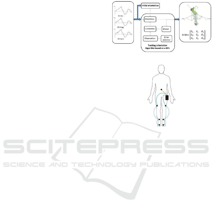
3.1 Capture System
Tech-MCS V3, a portable kinematics movement ac-
quire system was used to collect the database. This
system consists of a hub to store the data and 7 in-
ertial measurement units (IMU). Each IMU has one
accelerometer, one gyroscope and one magnetometer,
all of them work in 3D. The signals of each sensor
are merged to obtain the orientation of the IMUs. The
process is used in a sensorial fusion process in order
to obtain orientation using inertial information. This
process is performed by an Extended Kalman Filter
(EKF) that runs in each IMU. Diagram of the process
is presented in Figure 1. The orientation data can be
used to obtain the angle data of the joints.
To acquire the data, the seven IMUs were attached
the following way: two at the foot, two at the middle
of the shin, two at the middle of the sank and one at
the lumbar. In each walk, 81 signals were recorded.
The angle data correspond to different leg move-
ments. In Figure 3 the movements of each joint
are presented. The first one belongs to the sagittal
plane (x-axis), in which the flexion and extension take
place. The coronal plane (y-axis) is the next one; this
consists of the movement of the leg from right to left
and vice versa. The last one is the rotation of the joints
over themselves.
Figure 1: Process of the IMU to obtain the 3D orientation.
Figure 2: Positions of the IMUs in the body.
3.2 Protocol
A database of healthy and fake-pathological gait was
collected. In order to isolate the pathology studied
in this experiment, the people that collaborated did
not have any gait impediment, that means that no per-
son in the database suffers from sprains, surgeries, flat
foot, etc.
When simulating a pathology some points must be
taken into account.
1. Easiness and comfortability for the user.
2. Replicability for all users.
3. Similarity with real pathology.
Sprains can be simulated using a bandage. But is
not easy and, in some cases can cause some pain. Fi-
nally, clubfoot walk is simulated using sole padding.
In order to perform as real as a possible experi-
ment we consider the following rules:
• Comfortability: the users wear his/her own
clothes and shoes. The only restriction is not to
use high heels or flip-flops, due to it is not possi-
ble to use them with sole padding.
• Freedom: The users can perform the visit when
and wherever they want. The only restriction is
the walking path must be flat.
Recurrent Neural Network for Gait Pathology Detection
61
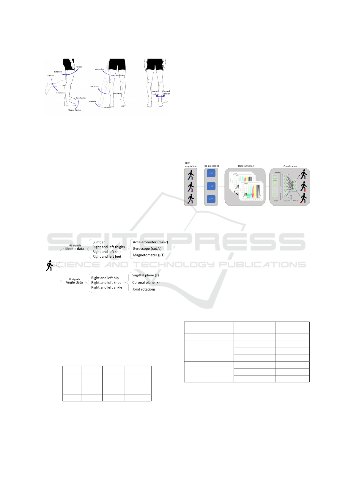
Figure 3: Different movements per plane.
Each user made three sessions, 15 days passed
from session one and two, and two months between
two and three. By doing this we eliminate variables
such as exhaustion or temporal pain in the users. Each
visit is made up of:
• 8 free walks.
• 4 walks with the sole padding in the right feet
• 4 walks with the sole padding in the left feet
3.3 Dataset
For this study, 31 healthy people were recruited. Of
these users, only 21 did the second visit, and of these
21 only 7 did the third one.
Figure 4: Schema of the recorded data.
As an addition, two people with an ankle sprain
(one on the right and the other one in the left) were
recruited for the experiment. Each user did 10 walks
walking freely. These people will be used at the end to
test if the system is capable of identifying real pathol-
ogy having been trained with fake pathology.
Table 1: Number of users, walks, and samples per visit.
Visit Users Walks Samples
1st 31 496 1984
2nd 21 336 1344
3rd 7 112 448
Total 59 994 3776
As we can see in 1 there are 3776 samples, 1888
are from healthy walks, and 944 from each left and
right limp walk. The ranged age of de database is
from 18 to 77 years old, and the gender distribution is
47 % female and 53%, male.
4 SYSTEM
The aim of the system is to distinguish between right-
limp walks, left-limp walks and no limp walks. The
system is divided into three steps. The first step is the
pre-processing, where the signals are filtered, once
the signal is filtered the signal is divided into frag-
ments. Lastly these fragments are classified using a
neural network. In Figure 5 the workflow of the whole
system is presented.
Figure 5: System workflow.
4.1 Pre-processing
Due to the nature of the gait signals, the bigger part
of the information is low frequency. So, to remove
unnecessary noise the signals were filtered by a But-
terworth low pass filter. The Butterworth filter is used
due to its simplicity and the -3 dB gain at the cut-
off frequency. We set the cut-off frequency, approx-
imately, in the frequency where the power spectrum
falls down under -40 dB. To find this frequency all
the signals were studied. Heuristically a group of dif-
ferent cut-off frequencies were obtained.
Table 2: Cut-off frequencies of the different signals.
Position Signal
Frequency
(Hz)
All Angle 20
Lumbar and thigh
Accelerometer 20
Gyroscope 10
Magnetometer 10
Shin and feet
Accelerometer 40
Gyroscope 20
Magnetometer 20
Once the signals are filtered the next step is to ex-
tract the data.
BIOSIGNALS 2020 - 13th International Conference on Bio-inspired Systems and Signal Processing
62
4.2 Data Extraction
Walking is a pseudo-periodic movement, this means
that it is almost the same movement every time: right
step, left step and repeat. These pseudo-periodic
movements are called gait cycles. In some studies,
these gait cycles are used as a basic unit for biometric
recognition (Fernandez-Lopez et al., 2018).
In this study, instead of gait cycles, a bigger part
of the data is used as a basic unit. By using fragments
larger than the gait cycles the evolution from the right
to the left and then from the left to the right step can
be observed, having much more information to locate
the pathologies.
• To avoid non-stable signal there must be at least
three seconds left before the start point. There
also must be three seconds left between the end-
point and the end of the signal;
• All the 81 signals of a walk must be trimmed using
the same points;
• The start and endpoint must be the same moment
in the cycle.
Once the constraints are fixed, the next step is to
perform the frame extraction. Since all the signals in
a walk are synchronized, the timestamps of all signals
are the same. This is why once we find the beginning
and end of a fragment in one signal the same times-
tamps are used to fragment the remaining 80 signals.
To choose the model signal, all the signals were
studied. The signals with the clearest cycles are from
the hip and the knee. There are not noteworthy differ-
ences between the signals from the right and the left,
so the right signals were selected. Once the lateral-
ity of the signals was selected, the signals of the hip
and the knee were inspected. The one with clearer re-
sults is the knee signal, this signal corresponds with
the flexion/extension movement. Thus, the right knee
signal is used as a model signal for the data extraction
process.
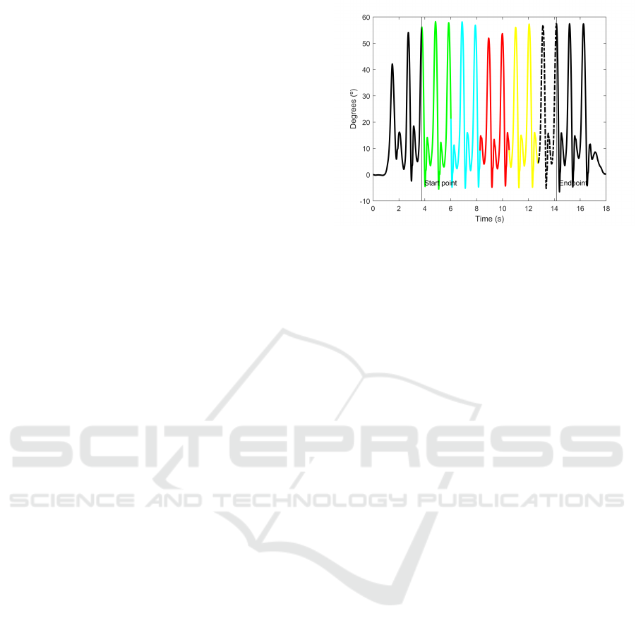
The first step of the extraction process is to seg-
ment the gait cycles. In this study, the maximum point
is used as the beginning of the cycle. This point cor-
responds to the position where the right leg is fully
stretched forward, that is, the knee has the greatest
extension angle. To find the proper maximum values,
and avoid the local maximum data, the peaks must
accomplish that:
• The distance between peaks must be greater than
900 ms (Fernandez-Lopez et al., 2017).
• The peak must be placed in the upper third.
Once the edges of the fragment are found, all the
signals in a walk are trimmed off in segments. After
Figure 6: Right knee signals. Different colours represent
different final fragments. Black and doted signal are dis-
carded.
the fragments have been obtained, the problem arises
from the fragments of each user and walk have a dif-
ferent duration. To solve this problem, all the signals
are trimmed to the length of the shorter one. Since the
signals still long enough, all of them are divided into
four segments.
In order to prepare the data to feed the neural net-
work, it has to be organised in samples. Each sample
is a matrix of N x 81 where N represents the number
of samples of the fragment. Each column represents
the different axis (x, y and z) and sensors (accelerom-
eter, gyroscope, magnetometer and body angles). Fol-
lowing is presented the organization of the data inside
the matrix.
Acc
x
(1) Acc
y
(1) Acc
z
(1) · · · LAnkle
x
(1) LAnkle
y
(1) LAnkle
z
(1)
Acc
x
(2) Acc
y
(2) Acc
z
(2) · · · LAnkle
x
(2) LAnkle
y
(2) LAnkle
z
(2)
Acc
x
(3) Acc
y
(3) Acc
z
(3) · · · LAnkle
x
(3) LAnkle
y
(3) LAnkle
z
(3)
· · · · ·· · · ·
· · · · ·· · · ·
· · · · ·· · · ·
Acc
x
(N) Acc
y
(N) Acc
z
(N) · · · LAnkle
x
(N) LAnkle
y
(N) LAnkle
z
(N)
4.3 Neural Network
With the aim of develop a neural network (NN), the
python deep learning library Keras (Chollet et al.,
2015) is utilised.
To feed the neural network (NN) the data is orga-
nized in a matrix. The output data corresponds to one
of the three cases of walk: no limp, left limp or right
limp.
A NN is a group of algorithms that attempt to rec-
ognize the relationship of a group of data through a
process that mimics the way the human brain oper-
ates. Depending on the data there are some NN that fit
better. In these algorithms, there are multiple options
for configuration. In order to obtain the better results,
the number of layers, the neurons of each layer, num-
ber of filters, the activation algorithm, ratio of train-
Recurrent Neural Network for Gait Pathology Detection
63
ing/testing, etc. can be set up. These adjustable pa-
rameters are called hyperparameters.
There is not a fixed rule about how many layers
should be used. Three layers are the minimum num-
ber of layers we can have. More layers can give better
results, but it will be harder to train. This study com-
pares the results and the training time of two neural
networks: the first one with three layers and the sec-
ond one with four layers. The number of neurons per
layer is also studied. To do this the relationship be-
tween the layers is fixed. The input layer has 2
n
neu-
rons. The hidden layers have 2
n−1
neurons. The out-
put layer never has 3 neurons, since it is the number
of classes to predict. The value of n starts in 2. The
value is increased by 1 until the results stop improv-
ing. Thus, the results of how changes the accuracy
with the complexity of the NN can be observed.
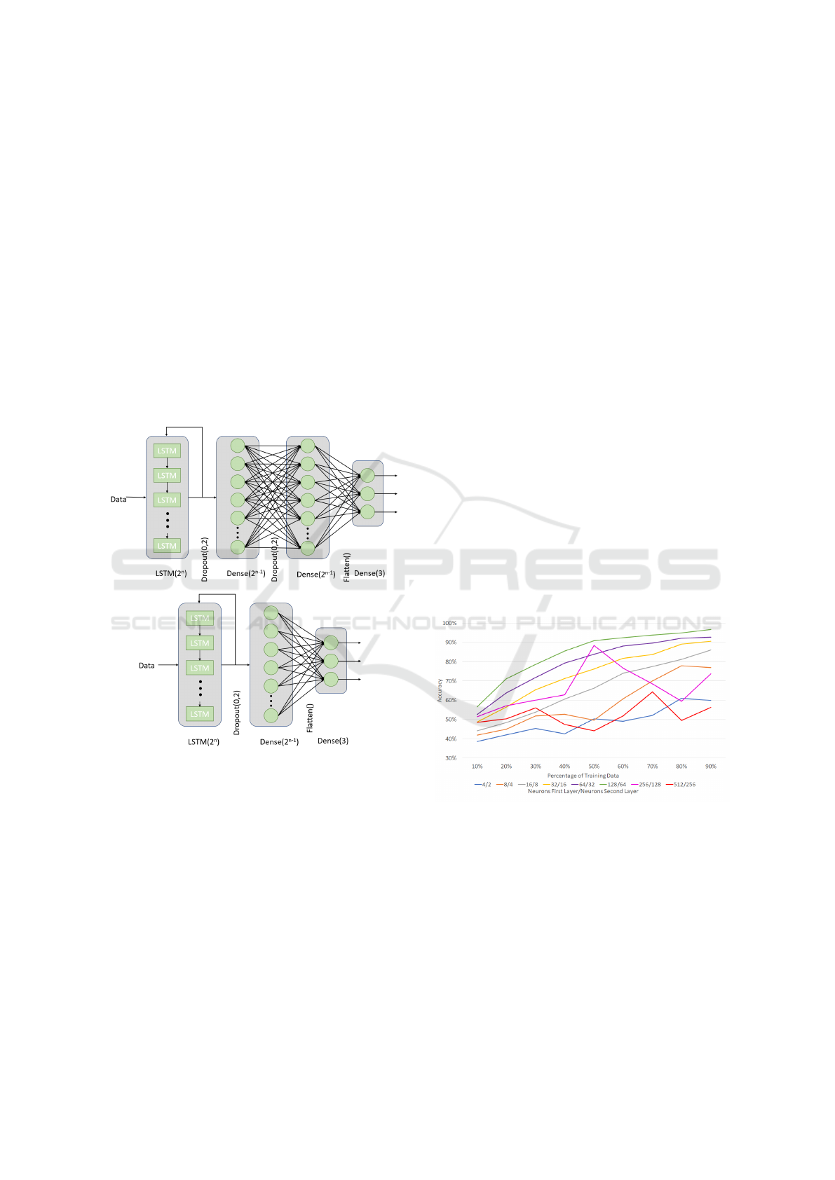
Figure 7: Structure of the neural networks.
Due to gait signals being temporal, a recurrent
neural network (RNN) (Hochreiter and Schmidhuber,
1997) is used. The structure of the three-layer NN is
shown in Figure 7. The input layer is an RNN with 2
n
Long Short-Term Memory (LSTM). The hidden layer
is a Dense layer and the output layer is a three neurons
layer. To avoid overfitting and improve the accuracy
of the system a dropout of 0.2 is performed after the
RNN layer. The structure of the four-layer NN is the
same, but it includes another dense layer between the
hidden layer and the output layer.
After each layer we use an activation function. Af-
ter the RNN and the hidden layers, we use relu, as it
maintains linearity. However, for the output layer, we
use a sigmoid function to get a probabilistic output.
In this study, to obtain the best results of the NN
the ratio of training/testing data and the number of
neurons in each layer have been analysed. The ratio
of train/test data goes from 10/90 % to 90/10 %.
5 RESULTS
The results of the different configuration of the sys-
tem are presented below. First case under study is
the effects of changing the ratin of raining/testing data
and the numbers of neurons per layer. Following this
the outcomes of adding an extra layer to the RNN are
presented. Two experiments have been performed: to
classify two real pathologies with the RNN and to
check if the system classifies equally right and left
walks. The results of these experiments are presented
at the end of the section.
The first parameter to study is the training-testing
ratio. In the state of the art, there is not a fixed ratio of
training-testing for the data, even though it is recom-
mended 20-40% for testing and 80-60% for training.
To solve this problem and to give a clearer solution,
we trained the network with different percentage of
data between 10 and 90%. For each ratio of data, the
algorithm has been trained and tested 10 times and the
final accuracy is the mean value of all of them.
Figure 8: Results of 3 layers network. Different colors rep-
resent different neurons per layer.
In Figure 8 and 9, we can see the accuracy of the
algorithm against the percentage of training data. In
general, a bigger training dataset provides better re-
sults. However, we can notice that there is a point
from which the increase of the training data does not
provide significant improvement. This point is lower
when the ratio of training data is bigger. For exam-
ple, in the network with n = 7 (128/64/64 neurons)
training with only 50% of the data, the 91% of the
frames are correctly classified,. However, if the train-
BIOSIGNALS 2020 - 13th International Conference on Bio-inspired Systems and Signal Processing
64
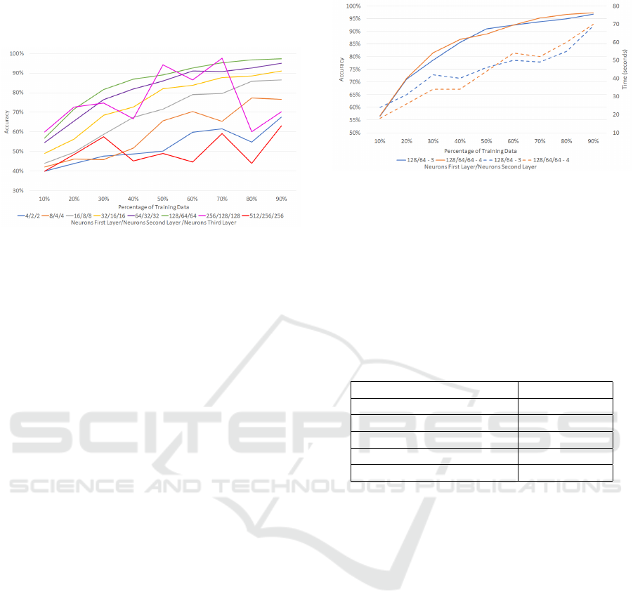
ing data is increased until 90% the accuracy only im-
proves 6%.
Figure 9: Results of 4 layers network. Different colors rep-
resent different neurons per layer.
A different number of neurons per layers has been
used in order to find the best configuration. The num-
ber of neurons per layer has been increased until the
improvement stops. As we can see in Figure 8 and 9
the accuracy grows with the number of neurons. The
more neurons the layers have, better the results. This
can be appreciated especially in the networks with
16/8, 32/16, 64/32 and 128/64. The optimal config-
uration occurs when n = 8 and it produces a network
with 256 neurons in the first layer and 128 in the sec-
ond and the third. The accuracy of this network does
not fit into any pattern. In Figure 8, the accuracy of
the network with a ratio of 50/50 of the data is 88%,
but it suddenly drops to 60% with a bigger training
dataset. This behaviour is due to the complexity of
the network as it is too high. On the other hand, the
networks with n = 2 and n = 3 have similar conduct,
but in this case, is due to not enough complexity.
Up to now, the best configuration is the one with
n = 7 and 90% of training data. The last hyperparam-
eter under study is the number of layers of the NN.
Two different NN have been created to determine the
influence of adding a layer: the first one with 3 layers
and the other one with 4. Figure 8 shows the results of
the 3-layer NN. The outcomes of the 4-layer NN are
presented in Figure 9. We can verify that the results
for both are similar.
Figure 10 presents the comparison of the best con-
figuration of NN with 3 and 4 layers and the training
time of each. As we can see the improvement in the
best case is lower than 3%. So, there is no significant
improvement adding an extra layer to the NN.
For all the possible configuration of the RNN
the one that offers the best results is the one with
128/64/64 neurons per layer and with 4 layers. In or-
der to test the RNN two experiments have been per-
formed: classifying walks of two users with sprain,
Figure 10: Comparison of the results with 3 and 4 layers.
The dotted line shows time. The solid line shows the accu-
racy.
and to check if the system classifies equally all the
cases.
For the first experiment two users with real ankle
sprain have been recruited. Each of these users has
done 10 walks, so 80 frames have been classified. The
results of classifying the frames are presented in table
3.
Table 3: Accuracy of classify sprain fragments.
Percentage of training data Accuracy (%)
50 % 45
60 % 50
70 % 66
80 % 71
90 % 83
The classification of the frames have been done
using the NN with 4 layers and 128/64/64 neurons
per layer. The network have been trained using the
fake pathology data, this network shows a result of
83% of accuracy classifying the samples. The drop
in the accuracy may be due to there are not sprains in
the training dataset. Even though it is not a negligible
result, it cannot be considered since the data used is
not enough.
The last experiment lies in to check if there is any
difference in the accuracy when classifying the differ-
ent walks separately. The network has been trained
with all data and tested only with the corresponding
cases. Seven cases have been studied: healthy walk
and left limp, healthy walk and right limp, either right
or left limp, only left, only right, only healthy and
all the walks. The accuracy against the ratio of train-
ing/testing data is presented in figure 11. The results
show that there is no significant difference when clas-
sifying the different cases.
Recurrent Neural Network for Gait Pathology Detection
65
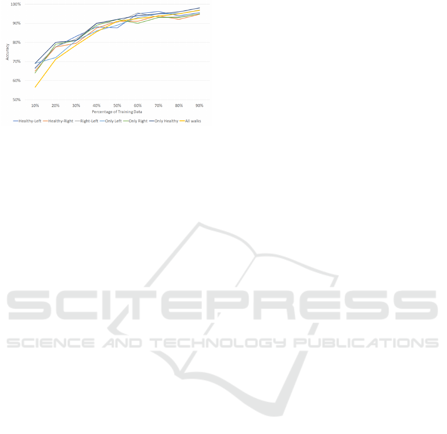
Figure 11: Comparison of classification the walks sepa-
rately.
6 CONCLUSIONS AND FUTURE
WORK
The aim of this paper is to present a system capable of
classifying pathology walks using RNN. The signals
of the lower train are recorded using a commercial
device, that records signals from accelerometer, gyro-
scope, magnetometer and orientation data. The sig-
nals are filtered and processed in order to extract the
information required to feed the neural network. With
the aim to obtain the optimal configuration of the NN
hand-tunning of the hyperparameters has been done,
among them the ratio of training/testing data, number
of neurons per layer and number of layers have been
studied.
To the light of the outcomes, we can see that, in
general cases, the accuracy of the system rises with
the training ratio. There are two cases where it is not
precise. This happens when the complexity of the NN
is too elevate, and the results do not converge at any
point. Adding an extra layer to the NN improves less
than 3% the accuracy of the system, however, it does
not increase significatively the effort.
The experiment of classifying the real cases of
pathology walks give proper results. However, the ex-
periment does not have a significant impact due to the
testing does not hold abundant data. Additionally, it
is able to classify equally the walks from the right and
left and the health walks.
Even though this system works and classifies
properly the walks, there are some improvements that
would be interesting to perform. The first one is to
study the influence of the origin (e.g. the beginning
or the middle of the walk) and the amount of data of
the fragments. In this way, if the amount of data can
be reduced without remarkable changes in the accu-
racy the algorithm can be optimized.
Once a system capable of distinguishing walk
limp and the laterality of them, the next step is to try
the system with real pathologies. So, the next step is
the acquisition of a new database of users with dif-
ferent problems in the lower train. In this case, the
algorithm should be refined to get as a result, not only
the laterality of the limp but also the joint where it
occurs.
ACKNOWLEDGEMENTS
This work was partially supported by the Spanish
National Cybersecurity Institute (INCIBE) under the
Grants Program “Excellence of Advanced Cybersecu-
rity Research Teams.”
The work of this paper has been partly funded by
PREVIEW project, granted by the Spanish Min-
istry of Economy and Competence, with the code
TEC2015-68784-R (MINECO/FEDER)
REFERENCES
Banala SK, Agrawal SK, S. S. (2007). Banala SK, Agrawal
SK, Scholz SP. Active leg exoskeleton (ALEX) for
gait rehabilitation of motor-impaired patients. IEEE
Int Conf Rehabil Robot 2007, 401–7. Rehabilitation
Robotics, . . . , 00(c).
Chollet, F. et al. (2015). Keras. https://keras.io.
Del Din, S., Godfrey, A., Galna, B., Lord, S., and Rochester,
L. (2016). Free-living gait characteristics in ageing
and Parkinson’s disease: Impact of environment and
ambulatory bout length. Journal of NeuroEngineering
and Rehabilitation, 13(1):1–12.
Dickstein, R. (2008). Review article: Rehabilitation of gait
speed after stroke: A critical review of intervention
approaches. Neurorehabilitation and Neural Repair,
22(6):649–660.
Fear, E. C., Li, X., Hagness, S. C., and Stuchly, M. A.
(2002). Confocal microwave imaging for breast can-
cer detection: Localization of tumors in three dimen-
sions. IEEE Transactions on Biomedical Engineering,
49(8):812–822.
Fernandez-Lopez, P., Sanchez-Casanova, J., Liu-Jimenez,
J., and Morcillo-Marin, C. (2017). Influence of walk-
ing in groups in gait recognition. Proceedings - Inter-
national Carnahan Conference on Security Technol-
ogy, 2017-Octob:1–6.
Fernandez-Lopez, P., Sanchez-Casanova, J., Tirado-Martin,
P., and Liu-Jimenez, J. (2018). Optimizing resources
on smartphone gait recognition. IEEE International
Joint Conference on Biometrics, IJCB 2017, 2018-
Janua:1–6.
Go, M., Iacovelli, C., Russo, E., Pournajaf, S., Blasi, C. D.,
and Franceschini, M. (2019). Stroke Gait Rehabilita-
tion : A Comparison of End-E ff ector , Overground
Exoskeleton , and. Applied Sciences.
BIOSIGNALS 2020 - 13th International Conference on Bio-inspired Systems and Signal Processing
66

Hausdorff, J. M., Rios, D. A., and Edelberg, H. K. (2001).
Gait variability and fall risk in community-living older
adults: A 1-year prospective study. Archives of Phys-
ical Medicine and Rehabilitation, 82(8):1050–1056.
Henriksen, E., Carlsen, J., Vejborg, I., Nielsen, M. B., and
Lauridsen, C. (2018). The efficacy of using computer-
aided detection (cad) for detection of breast cancer in
mammography screening: a systematic review. Acta
Radiologica, 60:028418511877091.
Hochreiter, S. and Schmidhuber, J. (1997). Long short-term
memory. Neural Computation, 8(8):1735–1780.
Kainz, H., Graham, D., Edwards, J., Walsh, H. P., Maine, S.,
Boyd, R. N., Lloyd, D. G., Modenese, L., and Carty,
C. P. (2017). Reliability of four models for clinical
gait analysis. Gait and Posture, 54(March):325–331.
Khouri, N. and Desailly, E. (2013). Rectus femoris trans-
fer in multilevel surgery: Technical details and gait
outcome assessment in cerebral palsy patients. Or-
thopaedics and Traumatology: Surgery and Research,
99(3):333–340.
M.H., T., G.C., M., and R.R., R. (1997). Rhythmic fa-
cilitation of gait training in hemiparetic stroke re-
habilitation. Journal of the Neurological Sciences,
151(2):207–212.
Moreau, N. G., Bodkin, A. W., Bjornson, K., Hobbs, A.,
Soileau, M., and Lahasky, K. (2016). Effectiveness of
Rehabilitation Interventions to Improve Gait Speed in
Children With Cerebral Palsy: Systematic Review and
Meta-analysis. Physical Therapy, 96(12):1938–1954.
Raveh, E., Schwartz, I., Karniel, N., and Portnoy, S. (2019).
Evaluation of the effectiveness of a novel gait trainer
in increasing the functionality of individuals with mo-
tor impairment: A case series. Assistive Technology,
31(2):106–111. PMID: 29035638.
Rutovi
´
c, S., Glavi
´
c, J., and Cvitanovi
´
c, N. K. (2019). The
effects of robotic gait neurorehabilitation and focal
vibration combined treatment in adult cerebral palsy.
Neurological Sciences, 40(12):2633–2634.
Schaafsma, J. D., Giladi, N., Balash, Y., Bartels, A. L.,
Gurevich, T., and Hausdorff, J. M. (2003). Gait dy-
namics in Parkinson’s disease: relationship to Parkin-
sonian features, falls and response to levodopa. Jour-
nal of the neurological sciences, 212(1-2):47–53.
Winter, D. A. (2010). The Biomechanics and Motor Control
of Human Gait. 74(2):94.
Yu, H., Riskowski, J., Brower, R., and Sarkodie-Gyan, T.
(2009). Gait variability while walking with three dif-
ferent speeds. 2009 IEEE International Conference
on Rehabilitation Robotics, ICORR 2009, pages 823–
827.
Recurrent Neural Network for Gait Pathology Detection
67
