
Model-to-Model Transformations for Efficient Time-domain Verification
of Concurrent Models by NuSMV Modules
Miguel Carrillo
1 a
, Vladimir Estivill-Castro
2 b
and David A. Rosenblueth
1 c
1
Instituto de Investigaciones en Matem
´
aticas Aplicadas y en Sistemas, Universidad Nacional Aut
´
onoma de Mexico,
Apdo. 20-126, 01000 Mexico D.F., Mexico
2
School of Information and Communication Technology, Griffith University, Brisbane 4111, Queensland, Australia
miguel.mcb@gmail.com, v.estivill-castro@griffith.edu.au, drosenbl@unam.mx
Keywords:
Model Checking, Kripke Structure, Value-domain Verification, Time-domain Verification.
Abstract:
We introduce and describe an algorithmic transformation from the formalism of arrangements of logic-labelled
finite-state machines (LLFSMs) into NuSMV modules (and its implementation as a model-to-model ATL
transformation from an Ecore meta-model to the NuSMV language). Our transformation benefits from using
modules and integers of NuSMV to improve the efficiency in the construction and verification of the model.
Moreover, we can handle predicates about time. Thus, we enable verification of LLFSMs in the time domain.
Our transformation is a considerable improvement in efficiency. Compared with earlier transformation algo-
rithms developed by us, the one presented here produces concise NuSMV files (in an example, 130,295 lines
were reduced to 418). We thus show that it is possible to automatically translate arrangements of LLFSMs to
concise models that can be efficiently and formally verified.
1 INTRODUCTION
We are concerned with model-driven software devel-
opment where the specification of a system is exe-
cutable. In practice, it does not suffice to have an exe-
cutable specification, as such a specification may also
contain errors. Although verifying non-executable
models brings insights into the correctness of the im-
plementation, errors can be introduced in the simpli-
fication of the executable program to a model, or the
implementation of a non-executable model into code.
Our objective is to show, within model-driven soft-
ware development, that it is possible to automatically
translate arrangements of LLFSMs to models that can
be efficiently verified with model checking.
We use logic-labelled finite-state machines (LLF-
SMs) to model and specify the behaviour of systems.
Earlier algorithms processing LLFSMs for model-
checking required the explicit construction (McColl
and Estivill-Castro, 2017; Estivill-Castro and Rosen-
blueth, 2011; Estivill-Castro and Hexel, 2013) of the
corresponding Kripke structure (Seshia et al., 2018,
Section 3.5, Definition 2). Our first contribution
in this paper is the application of model-to-model
a
https://orcid.org/0000-0003-2105-3075
b
https://orcid.org/0000-0001-7775-0780
c
https://orcid.org/0000-0001-8933-8267
transformations from an Ecore
1
meta-model to SMV
modules (Cimatti et al., 2000). Because we use the
SMV modules of NuSMV
2
, we obtain a tremendous
improvement in the efficiency of the description of the
verifiable model. For instance, for the four LLFSMs
of a microwave oven example, our NuSMV model
is only 418 lines long. The two separate implemen-
tations of our early algorithms, by contrast, deliver
NuSMV files for the same problem that have 130,295
lines one, and 110,567 lines the other. Work with the
earlier algorithms reports similar figures (McColl and
Estivill-Castro, 2017). These earlier algorithms suffer
also from not being able to use the native integers in
NuSMV (Cimatti et al., 2000). Such attempts, how-
ever, proved the first correctness results regarding no
overflow of the timer control for such an example. In
Section 3.4, we will show that the size of the output
of our algorithm is linear in the number of states of
1
Ecore is the first piece of the Eclipse Modeling Frame-
work for describing software models and meta-models.
2
In NuSMV’s language for describing Kripke structures,
modules are the fundamental tool for composability; default
composition of modules in NuSMV is synchronous (asyn-
chronous composition through processes is deprecated),
where a single step of the resulting Kripke structure cor-
responds to a simultaneous step of all component modules.
We will use “NuSMV” for the model-checker and “SMV”
for its input language.
Carrillo, M., Estivill-Castro, V. and Rosenblueth, D.
Model-to-Model Transformations for Efficient Time-domain Verification of Concurrent Models by NuSMV Modules.
DOI: 10.5220/0008910202870298
In Proceedings of the 8th International Conference on Model-Driven Engineering and Software Development (MODELSWARD 2020), pages 287-298
ISBN: 978-989-758-400-8; ISSN: 2184-4348
Copyright
c
2022 by SCITEPRESS – Science and Technology Publications, Lda. All rights reserved
287

the arrangement of LLFSMs.
Models with LLFSM are verifiable for value-
domain properties. Few properties can be verified in
the time domain, but only as bounded model check-
ing, that is, considering only a finite prefix of a
path that may be a solution to an existential model-
checking problem (Biere et al., 1999). Our second
contribution is to explicitly transform the behaviour
of an arrangement of LLFSMs using time predicates
into Kripke structures that includes explicitly timers
as modules. Thus, time-domain properties that ex-
plicitly mention time units are verifiable with a stan-
dard model checker, such as NuSMV (Cimatti et al.,
2000).
2 EVENTS VS BOOLEAN
EXPRESSIONS
Perhaps the most prominent modelling language
for model-driven software development is the Uni-
fied Modeling Language (UML). In UML, impor-
tant abstractions for behaviour are UML statecharts.
UML statecharts label transitions between states with
events. This is a common feature to state-based sys-
tems derived from Harel’s seminal introduction of
STATEMATE (Harel et al., 1990). Modelling tools,
such as OMT, were influenced by STATEMATE and
adopted the event-driven approach (Rumbaugh et al.,
1991). Executable state diagrams and tools from
ROOM (Selic et al., 1994) also became event-driven.
Event-driven semantics was disseminated with exe-
cutable state machines by QM (Samek, 2008). In-
ternational standards such as the Specification and
Description Language (SDL) for telecommunications
systems use event-driven communicating extended
finite-state machines for modelling behaviour (ITU-
T Study Group 17, 2002). Even tools for multi-
agent systems simulation, such as repast (Ozik et al.,
2015), adopt the event-driven view.
Modelling with event-driven statecharts has sev-
eral advantages, but many authors have already dis-
cussed important drawbacks (Mellor, 2000; von der
Beeck, 1994). A first drawback with event-driven
statecharts is the ambiguous loose-ends of the Run
Until Completion semantics. Although apparently
simple in that all new events are queued while han-
dling the current event, this already raises two alter-
natives for events caused by the current event. Such
derived events could either go at the end of the queue
(if they are considered new events) or could be at the
front of the queue (if they are considered causes of
the new event). In either case, if there is more than
one listener for the same derived event, then we break
the assumption that no two events happen at the same
time. Further drawbacks are the evaluation of expres-
sions or reading of variables. For example, should
the guard associated with an event that labels a transi-
tion be evaluated when the event happens or when the
event is de-queued? The first option implies running
code that interrupts the current event and violates the
Run Until Completion semantics, but evaluating the
guard much later than when an event occurred may
be completely inadequate for the intended behaviour.
Because of the mental load that this semantics im-
plies, UML scenarios using it are hard for humans to
resolve (Estivill-Castro and Hexel, 2019). Moreover,
UML’s variation points on event handling may result
in several alternative semantics for UML executable
models. (Besnard et al. (2018) report that the verifi-
cation of a (value-domain) property results in an error
when using FifoEventPool, but is successful when us-
ing OrderedList-DeferredEventPool.)
UML is effective in the design of systems where
the environment is unlikely to produce a shower of
events. Graphical User Interfaces (GUIs) are a good
example of the success of event-driven systems. The
reason is that a GUI user is unlikely to click in two
widgets without time gaps in between. However, this
is not the case for Cyber-physical systems, where
showers of events are common. Queues are a ma-
jor problem for event-driven system and fundamental
theorems have long-time existed regarding the impos-
sibility of confirming claims in the time domain or
for real-time systems (Lamport, 1984). Verification
of event-driven systems leads directly to the state-
explosion that typically blocks model checking be-
cause all possible permutations of the arrival of events
and their progress in queues need to be considered.
An alternative are Logic-Labelled Finite-State
Machines (for short LLFSMs, but also known as pro-
cedural state machines (Drusinsky, 2006, Page 51)).
LLFSMs enable concurrency under a prescribed
schedule: “because [the automaton] can access the in-
put symbols at any time, it can visit states as fast as we
wish” (Drusinsky, 2006, Page 15). These behavioural
models label transitions with Boolean expressions (or
predicates also called enabling functions (Cheng and
Krishnakumar, 1993)) and have a long trajectory in
verification (Devadas et al., 1991). LLFSMs can be
used beyond the realms of reactive systems as the
transitions can be queries to an expert/deliberative
system that determines whether the transition should
trigger or not (Estivill-Castro et al., 2016). They
have been used to formally verify more efficiently and
more effectively more properties than other methods
in the following examples: a microwave oven, a mine
pump, a power car-window, and an ambulatory pump.
MODELSWARD 2020 - 8th International Conference on Model-Driven Engineering and Software Development
288

2.1 Related Work
The deployment of critical fault-tolerant real-time
systems has had a sustained interest in linking mod-
els to verification (Poledna, 1996). In particular, for
model-driven software development, where models
are considered the primary artefacts of the software,
model checking becomes of the utmost importance.
For example, for the development of safety-critical
avionics software, there has been constant interest
in (Meenakshi et al., 2006) 1) tools that automatically
translate certain Simulink models into input language
of a suitable model checker, and 2) ensuring that the
size of the translated model is not excessive for ver-
ification. However, we emphasize that our goal is to
reduce what others have identified as the semantic gap
between models and code (Besnard et al., 2018). The
issue is that most model-checking activity verifies a
model that abstracts away some aspects of the running
software (Besnard et al., 2018). Such aspects are usu-
ally also relevant when design models are converted
into executable code. Moreover, diagnosis processes
are complicated since separate (sometimes even man-
ual) transformations into a formal language are per-
formed to enable formal verification (Besnard et al.,
2018). A long list of tools has been reviewed and each
displays such semantic gap or diagnosis difficulty to
some extent (Besnard et al., 2018, Section 7).
We illustrate the aspects of this gap by review-
ing STP (Clarke and Heinle, 2000), an approach for
converting STATEMATE statecharts into SMV. This
revision will also highlight our preference for LLF-
SMs. First, despite attempting to handle the funda-
mental composition notation of STATEMATE (that is,
hierarchical nesting), STP cannot handle inter-level
transtions (Clarke and Heinle, 2000; Bhaduri and
Ramesh, 2004). Remarkably, events are converted to
event-variables that have the value true for exactly
one SMV time step (that is, the translation is from
LLFSMs instead of STATEMATE) and compound
events (the events derived from an event) are treated
as plain Boolean variables. While model checking
will provide some insights about visiting states and
transitions, there is not action language. In contrast
with our modelling, moreover, there is no notion of
time. After one event, nothing can happen (no new
event, and no input can change), until the model is sta-
ble (Clarke and Heinle, 2000; Bhaduri and Ramesh,
2004). Thus, the verifications correspond to a mathe-
matical model that is not implementable. The seman-
tics assumes that event handling completes ahead of
any other event and event ordering is guaranteed by
the environment. Also the modelling assumes the en-
vironment behaves friendly and all non-determinism
is resolved by closing the system to a suitable choice
by the environment (user).
A review (Bhaduri and Ramesh, 2004) of several
other similar translations (to SMV or SPIN) shows
that a crucial issue in formal verification of statecharts
is their semantics (in some cases, for instance RSML,
the translation does not preserve the semantics). Most
of those translations reviewed suffer from the same
issues as STP: they eliminate events, treating them as
Boolean variables (and returning to LLFSMs), elimi-
nating all need to model the queueing of events, and
leaving aside timing issues. Most of them support
closed systems only (Bhaduri and Ramesh, 2004). If
the method/tool attempts to queue events, it is a trans-
lation to SPIN that suffers from other limitations (only
useful for deadlock detection, or only one statechart).
3 FROM ARRANGEMENTS OF
LLFSMS TO EFFICIENT
MODULES
We now provide an algorithm transforming an ar-
rangement of LLFSM into a set of SMV modules. We
first describe the tools supporting our argument that
such an algorithm produces a description of the verifi-
able model that is significantly more efficient than that
of earlier work. Next, we will discuss the obstacles
in mapping each LLFSM to a module in SMV. We
will reduce our problem to that of translating LLF-
SMs that only have blocks of code in their OnEn-
try sections (equivalently, they have no sections) and
where blocks of code in a state have no dependencies.
We follow this by the description of our algorithm to
transform LLFSMs where no transition has an AFTER
predicate.
3.1 The Tools and Implementations
In model checking, systems are categorised as open
or closed (Seshia et al., 2018, Page 88). Closed sys-
tems have no inputs, and are frequently those that are
formally verified. When dealing with an open sys-
tem, a corresponding closed system is used by com-
posing the open system with a model of its environ-
ment. In particular, if the open system were to re-
ceive an input supplied by a user, we adopt the con-
vention (and thus modelling the user) that the value
of the input variable is any non-deterministic value in
its domain. Thus, the corresponding Kripke structure
has, on a state reading an input, as many successor
states as possible values the input could receive. The
Kripke structure is then non-deterministic and mod-
Model-to-Model Transformations for Efficient Time-domain Verification of Concurrent Models by NuSMV Modules
289

els the fact that the environment can pick the value
arbitrarily without the control of the software.
An important property of LLFSMs is that they
are executable. Moreover, they are not only inter-
pretable, but can be compiled. The clfsm scheduler,
available for downloading,
3
enables extended LLF-
SMs where the action language is C++. We, how-
ever, will use a subset of IMP (Winskel, 1993) as the
action language, a simple imperative language, be-
cause the main purpose of this paper is to demonstrate
the transformations of the imperative statements (and
not of elaborate data structures or objects). We will
use IMP’s arithmetic expressions and Boolean ex-
pressions. However, from IMP’s commands we take
the empty command, the assignment and sequenc-
ing. What we exclude from IMP are two control
commands: the selection (if-then-else) and the iter-
ation (while-do). The reason is that both these con-
structs can be emulated by LLFSMs. Thus, by the
structured program theorem (also called the Boehm-
Jacopini theorem), LLFSMs are Turing complete.
We support this paper with the release of a LISP
interpreter of arrangements of LLFSMs. This demon-
strates that all models are executable. This interpreter
enables to run arrangements of LLFSMs where inter-
action reveals the open nature of the system. More-
over, this LISP interpreter has an option -k so it
can produce the corresponding closed Kripke struc-
ture using the methods mentioned in the introduction,
where all states and transitions of the state system are
listed. Thus, this option produces the closed system
for verification. In particular, its output is readable by
NuSMV (Cimatti et al., 2000) and then one appends
the corresponding value-domain CTL or LTL formu-
las to verify the closed but non-deterministic model.
This confirms that LLFSMs are both executable and
verifiable in the value domain. We additionally pro-
vide the following files.
1. The corresponding Ecore files that define the
meta-models discussed in this paper.
2. xmi files of examples of arrangements of LLF-
SMs (including the Microwave (Shlaer and Mel-
lor, 1992; Myers and Dromey, 2009) and the
Level-Crossing (Besnard et al., 2018)).
3. ATLAS Transformation Language (ATL) pro-
grams that implement the transformations de-
scribed in this paper.
All are downloadable from earlier site.
3
http://mipal.net.au/downloads.php.
3.2 LLFSMs with no Sections
The generic conversion of an LLFSMs model to SMV
modules requires that we determine precisely the
syntax and the semantics of LLFSMs. Therefore,
besides the implementations mentioned earlier, we
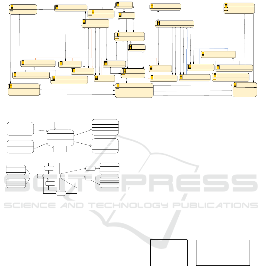
present here detailed definitions of LLFSMs. Figure 1
presents the Ecore meta-model for LLFSMs. We will
start the description of our transformation by men-
tioning two aspects where LLFSMs are analogous to
UML’s statecharts, and thus, adoption of LLFSMs is
accessible to UML users. First, we have already men-
tioned that in LLFSMs, each transition is labelled by
a Boolean expression, and not an event. Thus, users
familiar with UML will find that LLFSMs transitions
are labelled only by guards. Because transitions are
not labelled by events, the transitions out of a state S
are structured as a sequence (they are not just a set;
they have an order). The order of the transitions out
of S is the order of evaluation of the corresponding ex-
pressions. In particular, the second transition can only
fire if the guard of the first transition is false and its
own transition label evaluates to true. In general, the
guard of the i-th transition is ¬g
1
∧ ··· ∧ ¬g
i−1
∧ g
i
,
where g
j
is the guard of the j-th transition. It is im-
portant to observe that the behaviour designer does
not need to explicitly list this potentially long Boolean
expression. However, when translating such a guard
to a SMV module, the guard must be explicitly de-
fined.
Second, a state in LLFSMs has three sections
analogous to the states of UML’s statecharts, but LLF-
SMs’ semantics is more precise. The OnEntry sec-
tion corresponds to code that is executed only the first
time the thread of execution arrives at the state (from
another state). The OnExit section is executed when
a transition fires (its Boolean expression evaluates to
true), prior to any code in the target state. The Internal
section is evaluated only when the sequence of transi-
tions out of the state has been exhausted with none of
them evaluating to true. These sections can be consid-
ered syntactic sugar for state transition systems that
have no sections in their states. Nevertheless, Figure 2
illustrates the non-trivial translation we perform from
LLFSMs with states that do have sections, to LLF-
SMs with states that do not have sections. This also
needs to be made explicit, since the NuSMV model
checker needs to be explicitly alerted of the interme-
diate states of execution implied by the sections of
states. Figure 2 illustrates a state with sections, two
self transitions and two other transitions. The sections
imply that after the execution of the OnEntry, there
is a new state of execution for the other sections, so
that there is an asymmetry with the OnExit (Estivill-
MODELSWARD 2020 - 8th International Conference on Model-Driven Engineering and Software Development
290
variableID : Estring
maximumValue : EInt
[1..*]statements
[1..1]leftExpression
Section
OutputLine
1
stateName : EString
Tran sition
[1..1]targetState
AssignmentBooleanLHS
Statement
SimpleBooleanExpression
State
1
stateName : EString
BooleanConstant
1
aBooleanValue : EBoolean
[1..1]rightExpression
[1..1]leftExpression
BooleanExpression
StateMachine
1
name : EString
[1..*]stateMachine
Arrangement
1
arrangementName : EString
InitialState
[1..1]initialState
BooleanVariable
1
variableID : EString
[0..*]states
[0..*]transitions
[1..1]sourceState
[1..1]booleanExpression
[0..1]onEntry
[0..1]onExit
[0..1]internal
AssignmentIntegerLHS
[1..1]aBooleanExpression
ArithmeticExpression
[1..1]anArithmeticExpression
OrExpression
AndExpression
NotExpression
[1..1]leftExpression
[1..1]rightExpression
[1..1]notExpression
BooleanVariableReference
[1..1]theVariable
ListOfBooleanVariables
[0..*]variables
[1..1]variable
[0..1]booleanWhiteboardVariables
[0..1]booleanSensorVariables
[0..1]booleanEffectorVariables
IntegerVariable
1
1
[1..1]variable
ListOfVariables
TimeExpression
SimpleIntegerExpression
IntegerConstant
1
aBooleanValue : EBoolean
IntegerVariableReference
LessThanExpression
SubstractionExpression
AdditionExpression
[0..1]effectorVariables
[0..1]sensorVariables
[0..1]whiteboardVariables
[1..1]timeBound
[1..1]rightExpression
[1..1]leftExpression
[1..1]leftExpression
[1..1]rightExpression
[1..1]rightExpression
[1..1]theVariable
[0..*]variables
Figure 1: The meta-model that defines the behaviour models as an arrangement of LLFSMs for IMP.
other state 2
OnEntry O2A
OnExit O2B
Internal O2C
other state 1
OnEntry O1A
OnExit O1B
Internal O1CC
target state 2
OnEntry A
OnExit B
Internal C
target state 1
OnEntry T1A
OnExit T1B
Internal T1C
source state
OnEntry SA
OnExit SB
Internal SC
4:self
2:self
3:TST2
1: TST1
TO2S
TO1S
SB
SB
SB
SC
SB
SA
other state 2
OnEntry O2A
OnExit O2B
Internal O2C
other state 1
OnEntry O1A
OnExit O1B
Internal O1CC
target state 2
OnEntry A
OnExit B
Internal C
target state 1
OnEntry T1A
OnExit T1B
Internal T1C
true
true
5: not TST1 and not slef1 and not TST2 and not self2
true
true
true
4:self2 and not TST2 and not slef1 and not TST1
3:TST2 and not self1 and not TST1
2:self1 and not TST1
true
1:TST1
TO2S
TO1S
Figure 2: Illustration of the transformation that builds states
without sections from states with sections.
Castro and Hexel, 2019). And while OnExit code is
executed only on arrival from another state, self tran-
sitions do execute the OnExit, skip the Internal, and
ensure the state is not terminal (in LLFSMs, states
without exiting transitions are terminal). In what fol-
lows, we can assume that our models of behaviour are
LLFSMs with only actions in the OnEntry sections.
Along the same lines, is the translation of exe-
cutable blocks in LLFSMs. LLFSMs are Commu-
nicating Extended State Machines (Kang and Lee,
1993). They are extended because LLFSMs use vari-
ables in (assignment) statements in the sections of
states (and in the Boolean expression labelling the
transitions). Theoretically, the use of variables (from
an action language) is a technicality to avoid a large
number of states; but since our target SMV can ma-
nipulate integer and Boolean variables, we will use
variables of these two types.
LLFSMs are communicating because the vari-
ables can be shared between state machines of an
arrangement. The shared variables are called white-
board variables or external variables. Variables local
to a finite state machine are not shared.
Blocks of code in IMP (Winskel, 1993) are se-
quences of assignments of the form
hvariablei::=hexpressioni.
The assignments are typed. Thus, if the left-hand
side (LHS) is a Boolean variable, the right-hand side
(RHS) is a Boolean expression, and alternatively, if
the LHS is an integer variable, then the RHS is an
integer expression.
These blocks of code represent the next hurdle for
translating to SMV modules. If the sequence of as-
signments do not represent a dependency that causes
an intermediate state of computation, then the trans-
lation is direct. For instance, if the LHS of each as-
signment never appears in a later assignment, then the
sequence of assignments in a block translates directly
one to one to SMV code:
v
1
::= e
1
v
2
::= e
2
.
.
.
.
.
.
v
t
::= e
t
→
next( v
1
) = e
0
1
next( v
2
) = e
0
2
.
.
.
.
.
.
next( v
t
) = e
0
t
where e
0
i
is the translation of e
i
from expression in
IMP (and their operators) to expression in SMV.
If, however, the sequence of assignments displays
a dependency, in particular a variable on the LHS
appears in a later assignment on the RHS or the LHS,
we must perform a transformation that eliminates the
implicit sub-state of IMP. Algorithm 1 is the pseudo-
code of our ATL implementation, which uses a
dictionary of pairs (variable,latest-SMV-expression).
The dictionary keeps a history of assignments. For
instance, if we the first assignment is x := y + 1,
the dictionary has the pair h(x, (y + 1))i. If the next
assignment is z := x + 3, the dictionary is updated.
First, free variables in expressions are replaced by ex-
pressions in the current dictionary, and second the dic-
Model-to-Model Transformations for Efficient Time-domain Verification of Concurrent Models by NuSMV Modules
291

Algorithm 1: IMP-sequence to SMV.
1: procedure SMV(s:IMP-sequence,d:Dictionary):String
2: if s.isEmpty() then
3: return ‘’ The empty string
4: else if 1==s.size() or not s.tail().inLHS(s.LHS().variable) then
5: RHS is converted to SMV and free variables appearing in d replaced by
corresponding strings in d
6: return ‘next(’+s.LHS().variable+‘)=’+s.RHS.to-SMV-subs-free(d) + SMV(
s.tail(),d.update( s.LHS().variable, s.RHS.to-SMV(d ) ))
7: else
8: return SMV( s.tail(),d.update( s.LHS().variable, s.RHS.to-SMV(d ) ))
9: end if
10: end procedure
tionary updates its entries. Thus, the new dictionary
is h(x, (y + 1)), (z, ((y +1) + 3))i.
When the sequence s of IMP assignments is not
empty and of length 1, the translation to SMV is
a next clause of the corresponding variable on the
LHS, and the SVM result of binding the free variables
on the RHS using the dictionary (and replacing oper-
ators of IMP to SMV).
When the sequence s of IMP assignments is longer
than 1, we analyse the first assignment. If the corre-
sponding variable on the LHS appears later again on
the LHS, there is no output because we cannot have
two SMV-statements of the form “next(v)=” for the
same variable v. Only the last one will produce out-
put. We always process the tail of s recursively with
an updated dictionary. The dictionary accumulates
the expressions, and records all over-writes. In our
running example, if the third assignment is z := y +
x, the second entry in the dictionary is updated. Now
the dictionary is h(x, (y + 1)), (z, (y +(y + 1)))i.
An arrangement of LLFSMs is executed in a sin-
gle tread. The individual finite-state machines are ex-
ecuted concurrently, and in a predefined schedule. As
we already mentioned, this reduces the uncontrolled
concurrency of event-driven systems, and a signifi-
cant part of the state explosion for model checking.
In what follows, we assume that LLFSMs hold ex-
ecutable code only in their OnEntry section and that
code does not introduce sub-Kripke states (the assign-
ments of that code can be treated atomically).
The transformations steps described so far may
seem straightforward; however, they are far from im-
mediate when implementing them with ATL.The first
difficulty is the order in which to apply the transfor-
mations so that they are applied to every state (in the
case of flattening each state to having code on the
OnEntry section) and to every block (sequence of as-
signments) in such a way that there are no interme-
diate computational states. The second complexity is
that these transformations demand contextual infor-
mation. They cannot be applied to the state (or the
block of code) without knowledge of all the transi-
tions arriving and departing the corresponding state,
the expressions labelling those transitions, and the
scope of the variables involved.
This brings us to the point in our transformation of
how variables in the LLFSM correspond to variables
in the SMV modules we produce. While each LLFSM
will be translated into an SMV module, we assign
what we refer to as an owner module to each variable
(those that provide the capability to use integers and
Booleans and provided the adjective extended men-
tioned earlier). In the resulting set of modules, we
declare each variable with an SMV declaration in the
module that owns it.
Whether the variable is external or local, we as-
sign an SMV module as its owner. The assignments
do not require human intervention.
1. If a variable v is local to an LLFSM M, it has the
module for M as v’s owner.
2. If a variable v is external, and does not appear on
the LHS of any assignment, v is considered as be-
longing to the environment (an input or a sensor)
and the SMV model is closed, as discussed before
(but the variable v can non-deterministically adopt
any value in its domain at each Kripke state). Such
a variable v has as its owner an SMV module
named main (which would be also used for the
predefined schedule of the arrangement).
3. If a variable is external and appears on the LHS
of assignments but of only one LLFSMs, then we
assign the SMV module for M as the owner.
4. If a variable v appears on the LHS of assignments
in states of two or more LLFSMs, the SMV mod-
ule for v is the main module and those modules
having it (either on their LHS or RHS) receive it
as a parameter by reference.
This last point of the transformation may seem con-
tentions as, at first glance, an apparent race condition
could present itself if two or more LLFSMs in the ar-
rangement that write into a variable (they have it in
the LHS of some of their assignments) were to exe-
cute in parallel. Recall that SMV composes modules
under synchronous composability. However, we will
ensure that the semantics of LLFSMs (that a prede-
fined schedule, typically one turn for each LLFSM
in the arrangement) is enforced by the module main.
Thus, we preserve that only one LLFSMs executes a
ringlet (Estivill-Castro and Rosenblueth, 2011) in its
current state and only one LLFSM holds the current
turn. We stress that there is only one thread per ar-
rangement.
We deal now with the communicating feature of
LLFSMs. LLFSMs may read the values of exter-
nal variables on the RHS of their assignments. We
achieve this by identifying, for each LLFSM M, all
MODELSWARD 2020 - 8th International Conference on Model-Driven Engineering and Software Development
292

the variables on the RHS of all its assignments (in all
its states) of which it is not the owner. This set of vari-
ables, plus those from Case 4 above becomes a list of
formal parameters to the SMV module for M.
With these preliminaries, we can now complete
the description of our algorithm for producing a set
of SMV modules that corresponds to the behaviour
defined by an arrangement of LLFSMs. The merits of
the transformation are that it is (a) linear in the size of
the description of the arrangement and (b) completely
independent of the states of computation of the ar-
rangement (as opposed to our previous approaches).
3.3 Translating LLFSMs with no AFTER
We present our algorithm as a series of transforma-
tion steps which are analogous to ATL’s declarative
rules. However, for the purposes of illustrating this
presentation, we introduce a simple arrangement of
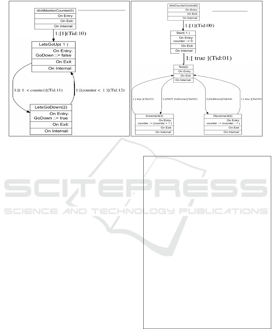
two LLFSMs (refer to Figure 3, which is drawn by our
ATL program transforming LLFSMs arrangements
into dot (Gansner et al., 2015) input).
An arrangement of LLFSMs with actions only in
the OnEntry section (such as the example in Figure 3)
can be thought of as an array of Christmas lights,
where only one arrow fires at each point in time, be-
cause there is a schedule (a pattern) that programs the
display. Figure 3 shows each LLFSM in a rectangle.
The LLFSMs scheduler assigns a turn to the arrange-
ment in round-robin fashion.
Transformation Step: Our SMV model will con-
sist of a module for each of LLFSM (total n) and a
main module with a variable turn. The domain of
turn is from 0 to n − 1.
Illustration: The code below is what our ATL
transformation produces for Figure 3, except that we
have here added the initialisation turn=0 (Line 6) to
the first LLFSM in the arrangement (but we typically
verify properties for any possible order of the LLF-
SMs in the arrangement).
1: MODULE main
2: VAR turn : 0..1;
3: VAR
4: CounterControl : CounterControl(turn ,
MonitorCounter.GoDown);
5: MonitorCounter : MonitorCounter(turn,
CounterControl.counter );
6: INIT turn=0
7: TRANS
8: ((turn = 0) & (next(turn) = 1 )) -- next
9: |
10: ((turn = 1) & (next(turn) = 0 )) -- next
Transformation Step: A module instantiation for
each LLFSM in the arrangement is listed in module
main with actual parameters identified with the prefix
of the owner (or no prefix, if main is the owner).
Illustration: The earlier code includes the decla-
ration of the two modules (Line 4 and Line 5) cor-
responding to the two LLFSMs in Figure 3. It also
shows the actual parameters. Both modules will read
the value of turn.
Transformation Step: The module main sched-
ules the variable turn so that the synchronous compo-
sition of modules by SMV results in only one module
advancing a step. The round-robin schedule is a series
of conditions
(turn = i) & (next(turn) = i mod n)
for i = 0, . . . , n − 2 and for i = n − 1
(turn = i) & ( next(turn) = 0 ) .
In general, for LLFSM M
i
, all the transitions in the
SMV module will have the test (turn = i). There-
fore, no transition fires in the SMV model, except for
a module whose turn is next, and main performs the
round-robin assignment of the turn.
Transformation Step: Not only LLFSMs are
numbered to be identified. The states within a
LLFSM are also numbered. Transitions are numbered
sequentially within a pair (i, j) consisting of their ma-
chine number i and their transition number j (and re-
specting their order when they share a source state).
Illustration: For example, state LetsGoUp is
State 1 in Machine 1 (MonitorCounter), while state
Decrement is State 4 in Machine 0 (refer to Figure 3).
So in Machine 0 (CounterControl), the transition
from Start to Test, the transition is Tid=01.
Transformation Step: Each machine M
i
will
have a program counter (pc) indicating its current
state, with values from 0 to the number of states in
M
i
. For a transition Tid=i j with label be
j
to fire, it
must be that it is the i-th machine’s turn, the program
counter is in the source state s of Tid=i j, the labelling
expression be
j
evaluates to true, and all other transi-
tions with the same source state as source do not fire
(remember that there is an order for transitions out of
the same state). For each transition Tid=i j with label
be
j
, we define conditions (in SMV)
condT
i j
:=(turn = i) & (pci= s) &be
j
.
When a transition Tid=i j fires, it has the consequence
of advancing the Kripke structure to the next Kripke
state with a new valuation. The first consequence
is the update of the program counter (the machine
changes state). The other consequence is the effects
of the block of assignment statements in the OnEntry
of Tid=i j’s target state. We emphasise one relevant
point: because of the semantics of SMV, for those
Model-to-Model Transformations for Efficient Time-domain Verification of Concurrent Models by NuSMV Modules
293
MonitorCounter
CounterControl
Figure 3: A small illustrative arrangement of two LLFSMs.
variables owned by the module and that are not as-
signed a value in the code block, we must explicitly
indicate that their valuation is not changing.
Illustration: Figure 4 shows the code generated
by our ATL implementation of the model-2-model
transformation. Line 3 shows that this module owns
variable GoDown. It is a whiteboard variable that ap-
pears in the LHS of statement in it. Line 5 starts the
definition of the conditions for what is the only possi-
ble transition that would fire when it is this module’s
turn. Note that the restrictions in TRANS ensure that a
transition fires only if no earlier transition fires. It also
shows the effect of the OnEntry of the target state, if
the transition fires. We also highlight the statement in
Line 25 where our algorithm explicitly indicates that
the Boolean variable GoDown is not changing value if
it is not this machine’s turn.
3.4 Complexity of the Algorithm
The construction presented earlier shows that for ar-
rangements of LLFSMs having only blocks of code in
the OnEntry sections and with no dependencies, the
resulting SMV models have exactly the same seman-
tics as the Ecore arrangements of LLFSMs.
The complexity of the output of the ATL trans-
formation is linear in the total number of states. Ob-
serve that there are as many lines in the DEFINE and
TRANS sections as there are transitions in the arrange-
ment. For each LLFSM the DEFINE and TRANS have
as many lines as transitions in the particular LLFSM.
The size of the output (in number of characters) is
1: MODULE MonitorCounter(turn, counter)
2: VAR pcMonitorCounter : 0..2;
3: VAR GoDown : boolean;
4: INIT (pcMonitorCounter = 0)
5: DEFINE
6: condT10 := ((((turn=1)&(pcMonitorCounter=0))&TRUE);
7: condT11 := ((((turn=1)&(pcMonitorCounter=1))&(1 <
counter));
8: condT12 := ((((turn=1) & (pcMonitorCounter=2)) &
(counter < 1));
9: condDefault1:= (!(condT10)& !(condT11)& !(condT12));
10: TRANS
11: (TRUE & -- Ncond
12: condT10 & -- Pcond
13: (next(pcMonitorCounter)=1)&(next(GoDown)=FALSE))
14: |
15: ( !(condT10) & -- Ncond
16: condT11 & -- Pcond
17: ((next(pcMonitorCounter)=2)&(next(GoDown)=TRUE))
18: |
19: ( !(condT10) & !(condT11) & -- Ncond
20: condT12 & -- Pcond
21: ((next(pcMonitorCounter)=1)&(next(GoDown)=FALSE))
22: |
23: (condDefault1 & -- Ncond
24: TRUE & -- Pcond
25: ((next(pcMonitorCounter)=pcMonitorCounter) &
(next(GoDown)=GoDown))
Figure 4: Machine 1 by our ATL m-2-m transformation.
quadratic in the number of transitions of the LLFSM
since for the i-th transition we must spell out that no
previous transition fires. Nevertheless, the reduction
in the size of the SMV files is several orders of mag-
nitude the length of the arrangement. For the small
MODELSWARD 2020 - 8th International Conference on Model-Driven Engineering and Software Development
294

SMV model of Figure 3, our ATL implementation
produces a SMV input file with 110 lines. By con-
trast, our earlier methods produce an SMV file with
820 lines.
4 TRANSFORMATION INTO
TIMERS
We now extend the transformation, so that time-value
properties can be verified with NuSMV. We will con-
trast value-domain properties with time-domain prop-
erties before we describe our modelling of timers.
4.1 What are Augmented LLFSMs?
The subsumption architecture for robotic and em-
bedded systems used LISP-coded LLFSMs (Brooks,
1990; Mataric, 1992). Such LLFSMs were aug-
mented because they use predicates about time. We
also discuss the implications of modelling time and
constructing Kripke structures for formal verification
with implicitly or explicitly time modelling.
The LLFSMs presented in the meta-model of Fig-
ure 1 are augmented and can be used for robotic and
embedded systems (Estivill-Castro and Hexel, 2018).
Such LLFSMs offer Boolean expressions of the form
AFTER(harithmetic-expressioni).
which can be part of the label of any transition. The
semantics of the AFTER Boolean expression for a tran-
sition T with source state s
1
and target state s
2
is that
a snapshot t
1
is taken of the system time when execu-
tion arrives at state s
1
(just before the execution of s
1
’s
OnEntry). At this time, the arithmetic expression that
is the argument of the AFTER is evaluated and the re-
sulting value ∆ is also saved. Execution of the ringlet
for s
1
proceeds as normal: the OnEntry is executed
and the transitions out of s
1
are evaluated in the order
of the sequence holding them. But when transition T
is evaluated, the AFTER is replaced by a comparison
of the current system time t
2
and the value t
1
+∆. The
AFTER evaluates to true if and only if t
2
> t
1
+ ∆.
4.2 Time-domain versus Value-domain
The original methods for verifying LLFSMs built
a Kripke structure (a SMV model) (Estivill-Castro
et al., 2012) where the AFTER is analogous to an en-
vironment variable. Then, the open model is con-
verted to a closed model as we mentioned earlier:
the Kripke structure offers non-deterministic tran-
sitions with both valuation (true and false) of the
AFTER. Thus, the verifiable properties are value do-
main properties. To illustrate this point we reproduce
the LLFSMs control of the ubiquitous Microwave
Oven (Shlaer and Mellor, 1992; Myers and Dromey,
2009). The Microwave Oven is analogous to the
Therac X-ray machine and has been widely discussed
in the literature of software engineering and formal
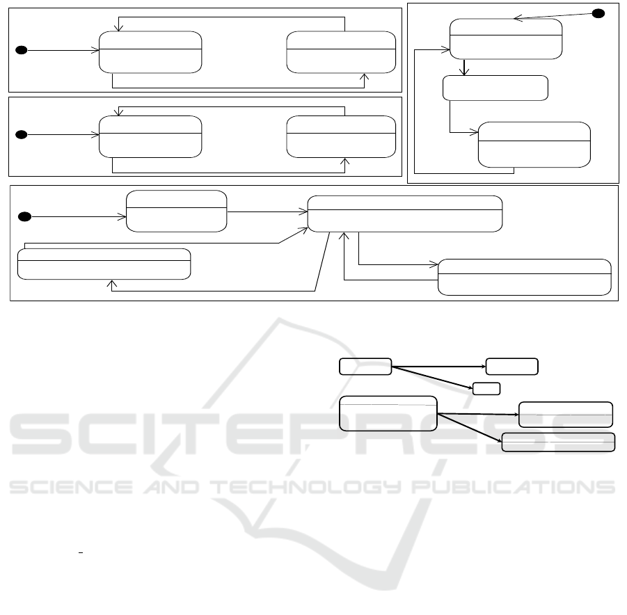
verification (Mellor, 2007). Figure 5 reproduces its
arrangement of LLFSM. There is a transition for the
bell-controller component with source RINGING to
BELL OFF that holds the sound effector active for two
units of time after the cooking has finished. There
is another transition in the time-controller with an
AFTER to decrement the time by 1 unit as long as the
door is closed and the button is released.
Value domain properties confirm desirable prop-
erties regarding the behaviour of the Microwave. We
find particularly illustrative that “After the sound ef-
fector is activated, eventually, the sound effector is de-
activated” (that is, the bell at the conclusion of cook-
ing does not ring forever). There is a symmetric prop-
erty that says that if the sound effector is silent and
cooking concludes, and the user does not add time
for some Kripke states, eventually the sound effector
rings. However, because of the construction of the
Kripke structure mentioned earlier, there is no way
to formulate a property that includes the value ∆ of
the argument of an AFTER predicate. The counts
of Kripke states are in the sense of bounded NuSMV
properties (that is, formulas require a precise number
of repetitions of the temporal logic operator X).
4.3 Transformation of Time
Expressions
We now propose to produce ATL transformations to
SMV modules where each appearing AFTER results in
a parameterised invocation to one timer module. The
timer module explicitly implements the test t
2
> t
1
+∆
as t
2
−t
1
> ∆. This means that
• the SMV model only uses integers as large as the
highest value for the arithmetic expression that is
an argument to an AFTER predicate;
• the integer variables about timers are SMV vari-
ables that can appear in CTL or LTL formulas.
Transformation Step: An instance of a timer (a
SMV module) interacts with the LLFSM M that labels
a transition T with source state s
1
and target state s
2
including an AFTER as follows. There are four shared
variables between the instance of the timer and the
SMV module for M. The first three are owned by M,
and thus parameters to the timer.
1. active: M sets active to true on arrival to s
1
.
Model-to-Model Transformations for Efficient Time-domain Verification of Concurrent Models by NuSMV Modules
295
LightControl
NoShineLightsState(1)
OnEntry:
LightsEffector::=false
ShineLightsState(2)
OnEntry:
LightsEffector::=true
1:[((NOT DoorOpenSensor) AND (NOT IsThereTimeLeft))](Tid:12)
1:[DoorOpenSensor OR IsThereTimeLeft](Tid:11)
1:[true](Tid:10)
TimerControl
DecreaseTimerState(4)
OnEntry:
CurrentTime::=CurrentTime-1
IncreaseTimerState(3)
OnEntry:
CurrentTime::=CurrentTime+60
InitialState(1)
OnEntry:
CurrentTime::=0
DecideIncrementDecrementState(2)
OnEntry:
IsThereTimeLeft::=(0<CurrentTime)
1:[(NOT ButtonPushedSensor](Tid:33)
1:[(((NOT DoorOpenSensor)AND
ButtonPushedSensor)AND((CurrentTime+60)<600))](Tid:32)
1:[true](Tid:35)
2:[(((NOT DoorOpenSensor) AND
IsThereTimeLeft)AND(AFTER 1)))](Tid:34)
1:[true](Tid:31)
1:[true](Tid:30)
BellControl
ArmedBellState(2)
OffBellState(1)
OnEntry:
SoundEffector::=false
RingingBellState(3)
OnEntry:
SoundEffector::=true
1:[(AFTER 2)](Tid:23)
1:[(NOT IsThereTimeLeft)](Tid:22)
1:[IsThereTimeLeft](Tid:21)
1:[true](Tid:20)
MotorControl
NotCookingState(1)
OnEntry:
MotorEffector::=false
CookingState(2)
OnEntry:
MotorEffector::=true
1:[(DoorOpenSensor OR (NOT IsThereTimeLeft))](Tid:02)
1:[((NOT DoorOpenSensor)AND IsThereTimeLeft)](Tid:01)
1:[true](Tid:00)
Figure 5: Complete executable and verifiable behavioural model (as LLFSMs) for the requirements (Shlaer and Mellor, 1992;
Myers and Dromey, 2009) of the Microwave.
2. bound: M assigns the value of the arithmetic ex-
pression to bound also on arrival to the state s
1
.
3. step: Also on entry to s
1
, M assigns this value
as required to decrement the local counter of the
timer per turn to the timer.
M makes active false in every target state of s
1
(not
only s
2
).
Illustration: For example, in the time-control of
the microwave, the user may push the button and
add even more time to a microwave already count-
ing down. In that case, the LLFSM moves to add time
when button pushed is true and abandons the wait-
ing for a second to pass to decrement the current time.
Transformation Step: The variable owned by the
instance of the timer is finished. This is set to false
at the start, but becomes true when the timer finds its
local time counter (which started at zero when ac-
tivated) reaches bound. The variable finished re-
places the predicate AFTER in the transition T .
Illustration: This model-2-model ATL transfor-
mation is illustrated in Figure 6. It is non-trivial as it
must be performed for each transition that holds one
or more AFTER predicates in the Boolean expression
that it labels them. Therefore, the set of variables for
each of these predicates are tagged by the machine
number, the Tid of the transition.
Transformation Step: An instance of the timer
module is created in the main module of the SMV
model. Only one generic timer module, a LLFSM
itself, is defined. But, as many instances as AFTER
predicates in the arrangement are constructed. They
become part of the SMV model and properties regard-
timer_finished
S
1
S
2
b
1
AFTER(bound)
S
1
S
2
b
1
S
3
S
3
timer_active ::= true
timer_bound ::= bound
timer_active ::= false
timer_active ::= false
timer_step ::= step
Figure 6: The transformation that replaces LLFSMs aug-
mented with AFTER-predicates to LLFSMs.
ing the behaviour of the arrangement and the bounds
in its AFTER predicates can be verified.
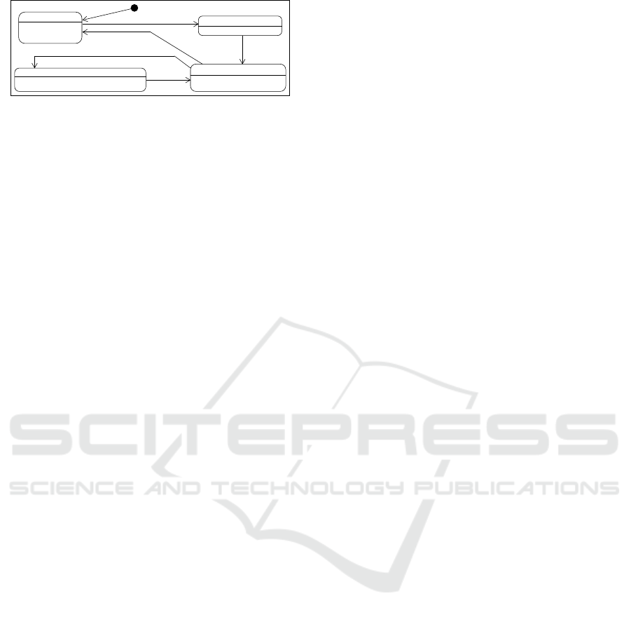
Illustration: Figure 7 shows the generic timer as
an LLFSM which we can produce in our LISP execu-
tion of LLFSMs for validation.
Transformation Step: The SMV module for the
only generic timer can be obtained by applying the
ATL transformation described in the previous section.
However, the ATL-transformation not only performs
the replacement of all the AFTER-predicates, but also
delivers one SMV generic timer module and the con-
struction of its instances in main.
Illustration: Figure 8 shows the snippet NuSMV
code in the main module resulting from the ATL pro-
gram applied to the executable model from Figure 5.
4.4 Complexity and Efficiency
Our ATL transformation delivers also a succinct SMV
when the executable LLFSM arrangement has AFTER-
predicates. The number of modules is the number of
LLFSMs in the arrangement plus one. The total num-
MODELSWARD 2020 - 8th International Conference on Model-Driven Engineering and Software Development
296
DecrementState(4)
OnEntry:
LocalCurrentTime::=LocalCurrentTime - step
GenericTimer
SetTimeBoudState(2)
LocalCurrentTime::=bound
InitialiseState(1)
OnEntry:
LocalCurrentTime::=0
finished::=false
TickTimeState(3)
OnEntry:
finished::=(LocalCurrentTime<1)
1:[(NOT finished)](Tid:t4)
1:[true](Tid:t5)
1:[finished AND (NOT active)](Tid:t3)
1:[true](Tid:t2)
1:[active](Tid:t1)
1:[true](Tid:t0)
Figure 7: The generic timer is also a LLFSM.
ber of instances of modules is the number of LLFSMs
in the arrangement plus the number of occurrences of
AFTER-predicates in the arrangement.
Using a desktop computer with an Intel quad-core
processor, 32 GB of RAM, and MacOS, it is possi-
ble to verify four properties that express requirements
of the microwave, in 551 s, 553 s, 853 s, and 853 s,
respectively, over NuSMV models generated by our
earlier algorithms (see the introduction). In contrast,
over the NuSMV model generated by the algorithm
of section 3, the same properties can be verified in
29 s, 32 s, 43 s, and 43 s, respectively, using a Ma-
cOS laptop with an Intel i7 processor and 16 GB of
RAM. We must highlight that, with some CTL prop-
erties, our earlier algorithms did not even finish after
running for one hour on the laptop.
4.5 Discussion
Time-domain properties are now expressible for SMV
directly. For example, SMV properties such as
CTLSPEC
AG( (0<=BellControlRingingBellState.LocalCurrentTime
& BellControlRingingBellState.LocalCurrentTime<=4)
& (0<= TimerControlDecideIncrementDecrementState.LocalCurrentTime
& TimerControlDecideIncrementDecrementState.LocalCurrentTime<=5)
)
that checks that the variable LocalCurrentTime, of
each timer instance, stays within respective bounds
is true (and the time required is minimal, because its
verification is tested by the compilation of the model
matching the bounds of the variable definitions).
Similarly, we can now revisit the discussion of
Section 4.2. As opposed to Kripke structures gener-
ated by closing the system when time predicates ap-
pear in the transition, now we can check specific real-
time properties.
EX (EF BellControlRingingBellState.LocalCurrentTime = 0)
EX (EF BellControlRingingBellState.LocalCurrentTime = 1)
EX (EF BellControlRingingBellState.LocalCurrentTime = 2)
are true, but
EX (EF BellControlRingingBellState.LocalCurrentTime = 3)
and larger values are false, showing the bell would
never ring for more than two time units.
The transformations discussed in Section 3 are
not necessarily completely equivalent regarding time
units in the micro-scale at which LLFSMs run. These
transformations (breaking the sections of a state into
separate states, for example) impact the predefined
schedule. The machine in question would need sev-
eral turns to complete for what was earlier a single
turn. Nevertheless, our methods provide the advan-
tage that such expansion of a few turns to one LLFSM
in the arrangement are conditions that should also
verified. Any arrangement of LLFSMs (executable
model of behaviour) that relies on specific timing
from subsections of states of participant LLFSMs for
fairness, liveliness or deadlock-free properties, is a
fragile behaviour design. Similarly, if the correctness
of the arrangement depends on the order of LLFSMs
in the arrangement, we will have a fragile design. Ver-
ifying these weaknesses in designs is now possible.
The efficient Kripke structures we are capable of pro-
ducing with the algorithms here enable verification
which previously was infeasible.
5 CONCLUSIONS
We have presented an algorithm (that is imple-
mented as an ATL model-2-model transformation)
that achieves succinct SMV models from generic ex-
ecutable forms of arrangements of LLFSMs. More-
over, this transformation enables involving time pred-
icates and later verifying properties about them, thus
extending the types of properties from the value do-
main to the time domain.
REFERENCES
Besnard, V., Brun, M., Jouault, F., Teodorov, C., and
Dhaussy, P. (2018). Unified LTL verification and em-
bedded execution of UML models. 21th ACM/IEEE
Int. Conf. Model Driven Engineering Languages and
Systems, MODELS ’18, p. 112–122, NY, USA. ACM.
Bhaduri, P. and Ramesh, S. (2004). Model checking of stat-
echart models: Survey and research directions.
Biere, A., Cimatti, A., Clarke, E., and Zhu, Y. (1999). Sym-
bolic model checking without BDDs. Tools and Algo-
rithms for the Construction and Analysis of Systems,
p. 193–207. Springer Berlin Heidelberg.
Brooks, R. (1990). The behavior language; user’s guide.
Tech. Rpt. AIM-1227, MIT, Dept. Electronics and CS.
Cheng, K.-T. and Krishnakumar, A. S. (1993). Automatic
functional test generation using the extended finite
state machine model. 30th Int. Design Automation
Conference, DAC ’93, p. 86–91, NY, USA. ACM.
Cimatti, A., Clarke, E., Giunchiglia, F., and Roveri, M.
(2000). NuSMV: a new symbolic model checker. Int.
J. Software Tools for Technology Transfer, 2(4):410–
425.
Clarke, E. and Heinle, W. (2000). Modular translation of
statecharts to SMV. Tech. Rpt., School of Computer
Science, Carnegie Mellon U., Pittsburg, PA.
Model-to-Model Transformations for Efficient Time-domain Verification of Concurrent Models by NuSMV Modules
297

VAR
OvenMotorControl: OvenMotorControl(turn,DoorOpenSensor, OvenTimerControl.IsThereTimeLeft);
OvenLightControl: OvenLightControl(turn,DoorOpenSensor, OvenTimerControl.IsThereTimeLeft);
OvenBellControl: OvenBellControl(turn,OvenTimerControl.IsThereTimeLeft, TimerOvenBellControlRingingBellState.finished);
OvenTimerControl: OvenTimerControl(turn DoorOpenSensor, ButtonPushedSensor, TimerOvenTimerControlDecideIncrementDecrementState.finished);
TimerOvenBellControlRingingBellState: Timer(turn, 4,2, 1,OvenBellControl.OvenBellControl RingingBellState active);
TimerOvenTimerControlDecideIncrementDecrementState: Timer(turn, 5,1, 1,OvenTimerControl.OvenTimerControl DecideIncrementDecrementState active);
Figure 8: The instantiation of modules in main for the SMV model of the executable model of Figure 5.
Devadas, S., Keutzer, K., and Krishnakumar, A. S. (1991).
Design verification and reachability analysis using al-
gebraic manipulation. IEEE Int. Conf. Computer De-
sign on VLSI in Computer &Amp; Processors, ICCD
’91, p. 250–258, IEEE Computer Soc.
Drusinsky, D. (2006). Modeling and Verification Us-
ing UML Statecharts: A Working Guide to Reactive
System Design, Runtime Monitoring and Execution-
based Model Checking. Newnes, Newton, MA, USA.
Estivill-Castro, V. and Hexel, R. (2013). Module isola-
tion for efficient model checking and its application to
FMEA in model-driven engineering. ENASE 8th Int.
Conf. on Evaluation of Novel Approaches to Software
Engineering, p. 218–225. SciTePress.
Estivill-Castro, V. and Hexel, R. (2018). Verifiable parame-
terised behaviour models - for robotic and embedded
systems. 6th Int. Conf. on Model-Driven Engineering
and Software Development, MODELSWARD, p. 364–
371. SciTePress.
Estivill-Castro, V. and Hexel, R. (2019). Resolving the
asymmetry of on-exit versus on-entry in executable
models of behaviour. 7th Int. Conf. Model-Driven
Engineering and Software Development, MODEL-
SWARD, p. 49–61. SciTePress.
Estivill-Castro, V., Hexel, R., and Ramirez Regalado, A.
(2016). Architecture for logic programing with ar-
rangements of finite-state machines. 1st CPSWeek
Workshop on Declarative Cyber-Physical Systems,
DCPS, p. 1–8. IEEE Computer Soc..
Estivill-Castro, V., Hexel, R., and Rosenblueth, D. A.
(2012). Efficient modelling of embedded software
systems and their formal verification. 19th Asia-
Pacific Software Engineering Conference, APSEC
2012, p. 428–433. IEEE.
Estivill-Castro, V. and Rosenblueth, D. A. (2011). Model
checking of transition-labeled finite-state machines.
Software Engineering, Business Continuity, and Ed-
ucation - Int. Conf. ASEA, p. 61–73. Springer.
Gansner, E. R., Koutsofios, E., and North, S. (2015). Draw-
ing graphs with dot.
Harel, D., Pnueli, A., Lachover, H., Naamad, A., Politi, M.,
Sherman, R., Shtull-Trauring, A., and Trakhtenbrot,
M. (1990). Statemate: A working environment for
the development of complex reactive systems. IEEE
Trans. Softw. Eng., 16(4):403–414.
ITU-T Study Group 17 (2002). Formal description tech-
niques (FDT) – Specification and Description Lan-
guage (SDL).
Kang, I. and Lee, I. (1993). A state minimization algorithm
for communicating state machines with arbitrary data
space. Tech. Rpt MS-CIS-93-07, Dpt. of Computer &
Information Science, U. of Pennsylvania.
Lamport, L. (1984). Using time instead of timeout for fault-
tolerant distributed systems. ACM T. on Programming
Languages and Systems, 6:254–280.
Mataric, M. (1992). Integration of representation into goal-
driven behavior-based robots. IEEE T. Robotics and
Automation, 8(3):304 –312.
McColl, C. and Estivill-Castro, V. Hexel, R. (2017). An
OO and functional framework for versatile semantics
of logic-labelled finite state machines. ICSEA : 12th
Int. Conf. on Software Engineering Advances, p. 238–
243. IARIA, Curran.
McMillan, K. L. (1992). Symbolic Model Checking — An
approach to the state explosion problem. PhD thesis,
Carnegie Mellon U., Pittsburgh, CMU-CS-92-131.
Meenakshi, B., Bhatnagar, A., and Roy, S. (2006). Tool for
translating Simulink models into input language of a
model checker. Formal Methods and Software Engi-
neering, p. 606–620, . Springer Berlin Heidelberg.
Mellor, S. J. (2000). UML point/counterpoint: Modeling
complex behavior simply. Embedded Systems Pro-
gramming.
Mellor, S. J. (2007). Embedded systems in UML. OMG
White paper. www.omg.org/news/whitepapers/ label:
We can generate Systems Today.
Myers, T. and Dromey, R. G. (2009). From requirements to
embedded software - formalising the key steps. 20th
Australian Software Engineering Conf. (ASWEC), p.
23–33, Gold Cost, Australia. IEEE Computer Soc.
Ozik, J., Collier, N., Combs, T., Macal, C. M., and North,
M. (2015). Repast simphony statecharts. J. Artificial
Societies and Social Simulation, 18(3):11.
Poledna, S. (1996). Fault-Tolerant Real-Time Systems: The
Problem of Replica Determinism. Kluwer, MA, USA.
Rumbaugh, J., Blaha, M., Premerlani, W., Eddy, F., and
Lorensen, W. (1991). Object-oriented Modeling and
Design. Prentice-Hall, NJ, USA.
Samek, M. (2008). Practical UML Statecharts in C/C++,
Second Edition: Event-Driven Programming for Em-
bedded Systems. Newnes, MA, USA.
Selic, B., Gullekson, G., and Ward, P. T. (1994). Real-time
Object-oriented Modeling. Wiley, NY, USA.
Seshia, S. A., Sharygina, N., and Tripakis, S. (2018). Mod-
eling for verification. , Handbook of Model Checking,
p. 1–26, Cham. Springer.
Shlaer, S. and Mellor, S. J. (1992). Object lifecycles: mod-
eling the world in states. Yourdon P., N.J.
von der Beeck, M. (1994). A comparison of statecharts vari-
ants. 3rd Int. Symposium Organized Jointly with the
Working Group Provably Correct Systems on Formal
Techniques in Real-Time and Fault-Tolerant Systems,
ProCoS, p. 128–148, Berlin. Springer.
Winskel, G. (1993). The Formal Semantics of Programming
Languages: An Introduction. MIT, Cambridge, MA.
MODELSWARD 2020 - 8th International Conference on Model-Driven Engineering and Software Development
298
