Evaluation of Reinforcement Learning Methods for a Self-learning

System

David Bechtold, Alexander Wendt, and Axel Jantsch

TU Wien, Institute of Computer Technology, Gusshausstrasse 27-29, A-1040 Vienna, Austria

Keywords: Reinforcement Learning, Machine Learning, Self-learning, Neural Networks, Q-learning, Deep Q-learning,

Replay Memory, Artificial Intelligence, Rewards, Algorithms.

Abstract: In recent years, interest in self-learning methods has increased significantly. A challenge is to learn to survive

in a real or simulated world by solving tasks with as little prior knowledge about itself, the task, and the

environment. In this paper, the state of the art methods of reinforcement learning, in particular, Q-learning,

are analyzed regarding applicability to such a problem. The Q-learning algorithm is completed with replay

memories and exploration functions. Several small improvements are proposed. The methods are then

evaluated in two simulated environments: a discrete bit-flip and a continuous pendulum environment. The

result is a lookup table of the best suitable algorithms for each type of problem.

1 INTRODUCTION

The interest in machine learning research has

exploded in recent years. Nowadays, it helps us to

accomplish tasks that could not be implemented from

scratch because of the immense state space. These

methods learn from experiences just as humans do,

but compared to us, much more additional data is

necessary. Human beings immediately recognize

which impact their actions have on the environment.

Machines lack that understanding. Due to the large

state space, the function to be learned is usually

approximated.

In a project, a self-learning agent shall be

developed that learns from scratch what its sensors

and actuators are doing and how to use them to reach

a certain goal. The overall purpose is to develop one

software that can adapt to an application, where the

interfaces to the environment are unknown at design

time.

A good approach to handle large state spaces is to

let the system learn to solve the task completely

independent. For scalability, the task should not be

tied to any assumptions about the environment.

Therefore, the agent should start with little prior

knowledge about the task, the environment, and the

meaning of the in- or outputs. In order for a new task

to be learned, only a reward function has to be

designed, which rewards the agent for performed

actions. With that in mind, a robot-like application is

appealing. For this, the following constraints should

be considered:

 Continuous state space, because sensory outputs

are continuous

 Work only with a partial part of the environment

perceived

 Deal with sparse rewards since real numbers are

uncountable

 Have as little knowledge about itself, the task and

the environment as possible

The agent has to predict which action to perform

next to receive a high amount of reward. Deep Q-

learning (DQN) performed well on several Atari 2600

games. DQN outperformed a linear learning function

in 43 out of 49 games and human game tester in 29

out of 49 games (Minh, 2013). Therefore, algorithms

from the area of reinforcement learning algorithms

are selected.

To prepare for a self-learning agent, the main

research objective of this paper is to address the

question: which combination of reinforcement

learning algorithms is most suitable for discrete and

continuous state spaces and action spaces.

The focus of this paper is to analyze, improve and

compare different Q-learning algorithms, replay

memories, and exploration functions to determine

which combination of algorithms to choose for each

task setting. The algorithms are being evaluated in

two simulation environments: a discrete bit-flip

Bechtold, D., Wendt, A. and Jantsch, A.

Evaluation of Reinforcement Learning Methods for a Self-learning System.

DOI: 10.5220/0008909500360047

In Proceedings of the 12th International Conference on Agents and Artiﬁcial Intelligence (ICAART 2020) - Volume 2, pages 36-47

ISBN: 978-989-758-395-7; ISSN: 2184-433X

environment (Andrychowicz, 2017) and a continuous

pendulum environment

2 AVAILABLE ALGORITHMS

Reinforcement Learning does not use labels for

datasets in the same way as supervised learning does.

There is no ground truth present. Instead, the agent

receives a reward or punishment signal through

exploration of an environment. It is attempted to

maximize this reward signal in the long-term because

the amount of reward describes how good or bad the

agent performed. Learning is described as finding

actions that result in a higher reward. Therefore, the

reward signal is transferred to an expected reward for

each state (Sutton, 1998).

There are two groups of methods: model-free or

not model-free. Not model-free methods require prior

knowledge about the environment in the form of state

transition probabilities. As this agent shall start from

scratch, only model-free methods are of interest.

A policy is a function, which maps states to

actions. The agent perceives a state. The policy

determines which action it will perform. In most

cases, the policy aims to maximize the cumulative

reward. On-Policy methods are based on known

policies. Off-Policy methods are based on learned

content.

Immediate rewards are given directly after an

action and no future rewards need to be considered.

To maximize the reward, only the selected action and

the current state of the agent are essential. Delayed

rewards mean that an action can generate immediate

rewards, but the future must be considered, at least

the next state of the environment. These problems are

more challenging to solve because the agent has to

choose actions that pay off in the future. Pure-delayed

rewards are the same for all states except the last state

of an environment. Playing chess, for example, could

be such a problem because the environment only

gives the agent a reward for winning or losing the

game.

Finally, the reward function can be designed to be

shaped or non-shaped. Non-shaped reward functions

usually provide only a positive reward for the main

goal of the task. Shaped reward functions are

typically designed to guide the learner towards the

main goal by providing rewards for getting closer to

the goal.

Open AI Gym; Pendulum, 2019.

https://gym.openai.com/envs/Pendulum-v0/

Reinforcement learning techniques try to solve

finite Markov Decision Processes (MDP). MDPs

describe the agent’s interaction with the environment

and vice versa. At each time step, the agent is located

in a state and performs an action selected by a policy

that leads to a successor state and receives a reward.

The goal is to optimize the total discounted

rewards over time. It requires a scalar number that

estimates how good it is to be in a specific state, or

which action should be performed next to receive a

high amount of reward. It can be achieved with the

help of the so-called state-value function and the

action-value function. The state-value function

provides the expected cumulative discounted reward

(expected return) for a state of a policy. The action-

value function provides the expected return for a state

executing the action of a policy.

2.1 Q-learning

Q-learning calculates Q-values, i.e. the expected

reward, which shows how much reward to expect by

performing a particular action from a certain state.

Deep Q-learning means that a neural net is used as a

function approximation for predicting the Q-values.

As a model-free algorithm is required, at least two

policies are usually used: one for exploring the

environment, e.g. a random policy, which updates the

Markov Decision Process of the agent. With this

knowledge, the second policy is used after training to

exploit the environment. When the state visits reach

towards infinity, the trained policy converges to the

optimal policy. At this point, the agent can stop

performing random actions and start to act according

to the trained policy.

An agent using the Q-learning approach updates

the corresponding Q-value after each observed

transition. A transition is a 4-tuple 



,



,



,





that consists of the current state 



, the performed

action 



, the resulting state 



and the earned

reward 



A method of updating the Q-values is the

Temporal Differences (TD) method (Dayan, 1992). A

problem with Temporal Difference Q-learning is that

Q-values must be stored in a lookup Q-table. For a

large continuous state space, it suffers from the Curse

of Dimensionality (Kober, 2012) and cannot be used

here. The team of Google DeepMind (Minh, 2015)

overcame this issue by using a neural network to

approximate the action-value function. Instead of

using a state and an action to update the Q-table with

Evaluation of Reinforcement Learning Methods for a Self-learning System

a Q-value, they only feed the Q-network with a state

and obtain a Q-value prediction for each action. The

highest Q-value represents the best action that can be

performed from a particular state. The Deep Q-

learning network (DQN) is trained with a loss

function that determines the error and allows the

weights to be changed. Further, a replay memory is

used to store the last n states, which are used as a

mini-batch for training.

A problem with DQN is that small changes in the

Q-values can lead to fast policy changes and thus, the

policy can begin to oscillate. It leads to an unstable of

the Q-values, which harms the task solving

performance. To prevent this particular case, the

Double DQN (DDQN) (van Hasselt, 2015) uses two

Q-networks: The first Q-network that is used for

action selection only and the second Q-network that

evaluates actions. It is attempted to keep the Q-

network as stable as possible over several transitions

by slowly updating its weights.

For robotic control, it is essential to consider

continuous action spaces. The predicted Q-values

only determine which action leads to the highest

amount of reward, but not with how much force this

action should be performed. (Lillicrap, 2015)

introduced the Deep Deterministic Policy Gradient

(DDPG), which introduces an actor-critic (AC)

algorithm to deal with continuous action spaces.

DDPG uses two Q-networks, of which one learns to

act (actor), while the other learns to criticize the taken

action (critic).

2.2 Replay Memories

All Deep Q-learning algorithms need to store

transitions in a replay memory. If this were not the

case, the Q-network would have to be trained by

successive transitions. It is like learning based only

on immediate experiences, without considering the

past. Experiences have to be considered to enable a

successful learning approach. It is done by saving

transitions in a so-called replay memory. However,

successive transitions are very inefficient due to the

strong correlation between them.

To break up these correlations, the transitions are

usually sampled randomly. Further, as the memory

gets full, the oldest transitions are deleted (Minh,

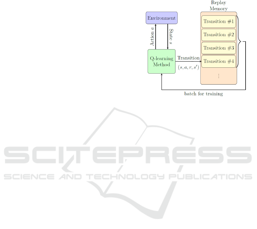
2013). The collaboration of the environment, Q-

learning method, and replay memory can be observed

in Figure 1.

An issue with this type of memory is catastrophic

forgetting (Kirkpatrick, 2017). Either it means that

the Q-network has learned a task correctly but forgets

about it by simply being trained with many useless

transitions, or it was not trained with transitions that

solve the task at all, i.e. in a sparse rewarding

environment.

Figure 1: Collaboration of the replay memory with the Q-

learning method and environment.

Experience Replay (EXPR) (Minh, 2013) is the

simplest and most widely used one. Transitions are

stored one after another in a memory of size N. The

most recent transitions experienced are always stored

at the end of the memory. Mini-batches are sampled

randomly distributed from the whole memory. As the

memory grows full, the oldest transitions, which are

the transitions at the beginning of the memory, are

deleted. Intuitively, this memory is the most

susceptible to catastrophic forgetting.

Prioritized Experience Replay (PEXPR)

(Schaul, 2015) takes advantage of the fact that the

temporal difference (TD) error of transitions can

easily be calculated. The TD error shows how

surprising or unexpected a transition is, i.e. the higher

the TD error of a transition, the more the agent can

learn from these transitions. Sampling only

transitions with high TD error can make a system

prone to overfitting, due to the lack of diversity.

Therefore, the TD error is converted to a priority. To

guarantee that even transitions with low priorities are

sampled with a non-zero probability from the

memory, multiple methods are used. One method is

to set the priority of a transition to the maximum for

the first insert. It ensures that these transitions are

sampled for sure in the upcoming mini-batch. Two

types of prioritizations are available: rank-based

(PRANK) and proportional-based (PPROP).

Hindsight Experience Replay (HER) is suitable in

a sparse reward environment. Rewards are only given

if a goal is reached (pure-delayed rewards). Usually,

multiple entire episodes are stored in the memory

without any positive rewards (Andrychowicz, 2017).

ICAART 2020 - 12th International Conference on Agents and Artiﬁcial Intelligence

From episodes without positive rewards, the Q-

learning approach only learns which actions should

not be performed. It is not useless knowledge, but in

the end, it does not help to solve the task. Therefore,

Q-learning learns little or even nothing from such

episodes. However, these episodes contain some

useful information, such as how non-goal states can

be reached. This knowledge is useful and can help the

agent to solve the task better and faster. If this state

must be visited in order to solve the task, the

knowledge about how to reach it can be considered as

relevant. To enable learning, the algorithm defines a

state as a virtual goal, rewards it with zero, and adds

it to the memory. As Hindsight Experience Replay

only instructs how virtual goals are generated and not

how to save them, it is compatible with all other

replay memory methods, like Experience Replay. To

decide which goal the Q-network should follow, the

state of the virtual or main goals is additionally

provided as an input. It makes it necessary to double

the size of the Q-network. Providing the main goals

as an input for the Q-network is, in the authors’

opinion, not suitable for self-learning. The Q-network

simply learns that it must reach the state, which is

equal to the goal input. Another issue is that HER

performs poorly in combination with shaped reward

functions (Andrychowicz, 2017).

2.3 Exploration

To learn policies in an optimal way, an agent must

make two far-reaching decisions: how long should the

environment be explored and when should it be

exploited? Exploration means that an agent performs

actions to gather more information about the task and

the environment. Exploitation means that an agent

only executes the best action possible from a certain

state. Finding out when to explore and when to

exploit is a key challenge, known as the exploration-

exploitation dilemma (Sutton, 1998).

Exploration methods can be divided into two

groups: directed and undirected (Thrun, 1992).

Directed exploration uses information about the task

and/or the environment. One requirement mentioned

in the introduction is that the agent should know as

little as possible about the task and the environment

at the start. Therefore, only undirected exploration is

considered here.

ε-greedy (EG) is a non-greedy exploratory

method in which the agent chooses a random action

with a probability of 0ε1at each time step

instead of performing the action with the highest Q-

https://gym.openai.com/envs/

value. To avoid the exploration-exploitation

dilemma, ε is decreased at each timestep by a fixed

scalar number. The main challenge is to find the right

exploration decline.

For a physical environment with momentum, an

Ornstein-Uhlenbeck process (OU) is usually used as

additive noise to enable exploration. This process

models the velocity of a Brownian particle with

friction (Lillicrap, 2015). Especially in the case of

robot control, such a process is used, due to the

drifting behavior of the output values. The parameters

can be set to produce only small drift-like values. In

general, the Ornstein-Uhlenbeck process is a

stochastic process with medium-reversing properties

as in equation 1.









 



∙













(1)

where 



.  means how fast the variable reverts

towards the mean.  is the degree of the process

volatility and  represents the equilibrium or mean

value and a is the start value of the process, which are

usually set to zero. The Ornstein-Uhlenbeck process

can be considered as a noise process. It generates

temporarily correlated noise. The noise ,,,

is added to the action to enable exploration.

3 RELATED WORK

Although reinforcement learning is a hot topic,

finding articles, which use real physical robots that

learn to solve problems on their own is rare. Dozens

of articles and simulation environments exist. For

example, the OpenAI Gym

offers more than sixty

environments in which learning algorithms can be

evaluated and compared to the results of other

competitors. However, not many articles deal with

few sensors and a reduced perception of the

environmental state.

Since robotic tasks are often associated with

complex robot motion models, poor environmental

state resolution and sparse rewards play an important

role. (Vecerik, 2017) introduces a new methodology

called Deep Deterministic Policy Gradient from

Demonstrations (DDPGfD) that should help to solve

those issues. The idea is to store a defined number of

task solving demonstrations in the replay memory and

keep them forever.

In to a 2D aerial combat simulation environment

with near continuous state spaces (Leuenberger,

2018), the Continuous Actor-Critic Learning

Automaton (CACLA) is applied. They replaced

Evaluation of Reinforcement Learning Methods for a Self-learning System

Gaussian noise by an Ornstein-Uhlenbeck process as

an exploration function and introduced a modified

version the Monte Carlo CACLA, which helped to

improve performance.

In (Shi, 2018), an adaptive strategy selection

method with reinforcement learning for robotic

soccer games was introduced. The researchers used

Q-learning to learn which strategy small robots

should follow in certain situations to successfully

play football. Each team consisted of four robots and

the game state was observed with a camera filming

the entire football field. The main issue addressed by

this work was that a very dynamic environment, such

as soccer with multiple teammates, requires timely

and precise decision-making.

In (Hwangbo, 2017), a reinforced learning

method was introduced for the control of a quadrotor.

The 18-dimensional state vector of the quadrotor

included a rotation matrix, the position, the linear

velocity, and the angular velocity. The policy was

optimized with three methods: Trust Region Policy

Optimization (TRPO) (Schulman, 2015), DDPG

(Lillicrap, 2015), and a new optimization algorithm

developed by the authors. While TRPO and DDPG

performed poorly, the algorithm of the authors

performed well. However, the authors used a model-

based learning approach, which is not applicable here.

(Tallec, 2019) analyzes how various parameters in

DDPG can be tuned to improve the performance in

near continuous time spaces. These are discretized

environments with small time steps. Through a

continuous-time analysis, where the time step is

considered, such as discount factor, reward, learning

rate and exploration parameters.

4 IMPROVEMENTS

For the particular problem of learning from scratch,

three improvements of the analyzed algorithms are

proposed. The aim is to achieve better results overall.

4.1 Hindsight Experience Replay with

Goal Discovery

The idea behind Hindsight Experience Replay with

Goal Discovery (HERGD) is that the main goal of the

agent has to be discovered first and only after its

discovery, it is provided to the Q-network. This

approach offers more flexibility than the standard

Hindsight Experience Replay, in which the main goal

has to be provided to the Q-network from the

beginning. Virtual goals are inserted as defined in the

standard Hindsight Experience Replay algorithm.

In environments where it is unlikely that the target

will be reached with random exploration methods,

HERGD will struggle in the same way as the ε-greedy

and Ornstein-Uhlenbeck process. Although, once the

goal is found, this approach can get to the optimal

policy faster.

4.2 ε-greedy Continuous

Since ε-greedy is only applicable to integer actions,

ε-greedy Continuous (EGC) extends the idea of

standard ε-greedy to support continuous action spaces

as well. The key idea behind this approach is that

every action from the action space has its own action

range [



,



]. For each action a, a random

uniform value  is drawn, for which 









is valid. The policy equation (2) tells when to

use a random action or a policy action.











    ∈ 







,



   







,

(2)









is the policy, 







is the action space and ε is

the threshold of exploration that is lowered with each

time step.

4.3 Ornstein-Uhlenbeck Annealed

An issue concerning the standard Ornstein-

Uhlenbeck process is that switching from exploring

to exploiting is done immediately. This means the

process is outputting noise until the exploration stops

and the exploitation begins. It can harm the learning

process because actions, that are already optimally

learned, can be overwritten by the outputted noise. On

the other hand, limiting the outputted noise by

adjusting θ or σ leads to under-exploration.

Therefore, the idea behind Ornstein-Uhlenbeck

Annealed (OUA) is to reduce the generated noise

after every time step by a function similar to ε-greedy

continuous as shown in equation 3









∶ 







 ,,,∙





(3)

For this evaluation, the function 







is selected to

reduce the noise linearly after every timestep.

5 EVALUATION

The algorithms are being tested for suitability and

being compared in different environments.

5.1 Experiment Environments

A discrete and continuous state environment is

provided to evaluate the algorithms. For both

ICAART 2020 - 12th International Conference on Agents and Artiﬁcial Intelligence

environments shaped and non-shaped rewards are

analyzed.

5.1.1 Discrete Bit-flip Environment

The basic idea of this environment is based on the bit-

flip environment (Andrychowicz, 2017). The goal is

to flip the bits in a bit vector 



of length n in the

same way that it matches a target bit vector 



within n tries. The state 





…





 is the

bit vector 



. The action a is the number of the

bit to flip and it can be chosen from the action space





0,1,…,1



. For instance, an action a = 2

means that the bit 





in bit vector 



is flipped.

To make the algorithms and methods comparable, bit

vector 



is always reset to zero and the target bit

vector 



is taken from a look-up table.

Minor adjustments had to be made to use this

environment for this application. Since DDPG

outputs continuous values and the bit to be flipped

must be an integer number, a conversion from real to

natural numbers has to be made. Therefore, the output

of DDPG is divided into n equal sections, each

representing one bit in the bit vector.

Because this is a discrete process, the Q-learning

method DDPG does not use an OU process for

exploration. Thus, only continuous ε-greedy

exploration is used.

In the non-shaped reward function, the reward for

reaching the goal is set to 1, and all other rewards are

set to -1. It simulates a delayed and sparse rewards

problem, since the probability of finding the target bit

vector 



is drastically decreasing with the bit

vector length n.

The shaped reward function simply counts the

equal bits of a bit vector 



and target bit vector





. Then, the counted number is divided by n-1.

5.1.2 Continuous Pendulum Environment

To be able to evaluate the RL methods within a

continuous action and state-space environment the

pendulum environment from open AI Gym was

chosen. The goal is to swing a frictionless pendulum

upright, so that it stays vertical, pointing upwards.

Figure 2 shows the pendulum near the maximum

reward position. The perceived state of this

environment is a three tuple ∈









,sin,. This state is generated by the

pendulum angle  and vertical velocity  of the

pendulum. To its state, a torque 22 can be

provided as an action a. However, to make this

environment more difficult to solve, the torque is

limited to 11 here. Therefore, the pendulum

must gain velocity through swinging to reach a

rewarding position. After a reset, the pendulum starts

in a random position and with a random torque.

Figure 2: The pendulum environment with the pendulum

position near the maximum reward position.

Non-shaped rewards are set to 1 if the pendulum

points upwards and its angle is in range of 1° 

1°. If not, the reward is set to -1.

For shaped rewards, this environment uses

equation 4 with   



 and 8   8.

Therefore, the reward is in the range of 16.27 

0.







0.1∗ 



0.001∗

(4)

Since Q-learning algorithms output discrete

actions, conversion from natural numbers to real

numbers is done. The output layer of DQN and

DDQN are extended to 21 nodes. Each of them

represents a specific torque value, starting from -1.0,

with a step size of 0.1, to 1.0 including zero.

5.2 Test Setup

A Q-learning method requires the following methods

to work: A Q-algorithm, an exploration method, a

replay memory, and a reward function. The Q-

learning algorithm can be considered as the brain.

Learning and decision making is done here. DQN and

DDQN use standard feed-forward multilayer neural

networks. Important parameters are the number of

layers and neurons, the activation functions, the

optimizer, the learning rate, the discount factor, and

the soft target update factor. The soft target factor is

only required for DDQN and DDPG because DQN Q-

networks do not include a second neural net.

According to (Lillicrap, 2015), all Q-networks in this

work use the Adam optimizer (Kingma, 2014).

The learning rate is multiplied by the values

computed by the optimizer. Therefore, it determines

how fast the Q-network learns. Since some of our

evaluations have to deal with sparse rewards, which

means that the past experiences are important, the

discount factor is chosen to be 0.98, which is close to

1.0. The learning rate and soft target update factor are

Evaluation of Reinforcement Learning Methods for a Self-learning System

chosen to be small, i.e. 0.001, because solving sparse

reward problems requires many transitions, since the

rewarding state is not often experienced. All hidden

layers use RELU units as activation function, as they

are currently the most successful and widely used

(Ramachandran, 2017).

For the replay memory, the most essential

parameter is its size. It determines how many

transitions can be stored. While large memory sizes

can only slow down learning, too small memory sizes

can drastically reduce learning success or even make

it impossible. Sizes from 16 to 128 state transitions

will be tested.

For the Hindsight Experience Replay,

additionally, the sampling method and the quantity of

new goals to sample has to be chosen. Based on

(Andrychowicz, 2017), the sampling method future is

selected because it gives the best overall results

together with the best value for parameter k = 4. For

PPROP, (Schaul, 2015) mentioned that a good value

for the prioritization factor is 0.6.

When exploring, it is sometimes necessary to

carry out already learned actions to be able to refine

them further and finally to solve the task in the best

way possible. For the exploration function, the most

critical parameter here is the exploration rate, which

determines after how many actions performed the

exploration ends and the exploitation begins. It is

common practice to place this value at the end of the

entire learning procedure, i.e.   ∗





The evaluations are carried out with Keras

framework, which is programmed with Python. It is

used to model neural networks and runs on top of the

symbolic math library TensorFlow

5.3 Results

The measurements are performed in two separate

environments: a discrete bit-flip and a continuous

pendulum environment

5.3.1 Discrete Bit-flip Environment

The evaluation starts with a bit vector length of n = 1.

At the end of each episode, which is exactly after 200

bit flips, it is checked if the current method solves the

bit vector with length n within n bit flips. If so, the

current attempt t is considered as successful. An

attempt t is assumed to be failed if a method fails to

solve a certain bit vector within 50 episodes. After

determining whether the bit vector length n has been

https://keras.io

solved successfully or the attempt has failed, the

method is reset and the next attempt t = t+1 is started.

After five tries, it is checked if the current method

has at least one successful attempt. If this is the case,

the next bit vector of length n := n + 1 can be

performed. The success rate of a reinforcement

learning method can be calculated by dividing the

total successful attempts by the number of attempts.

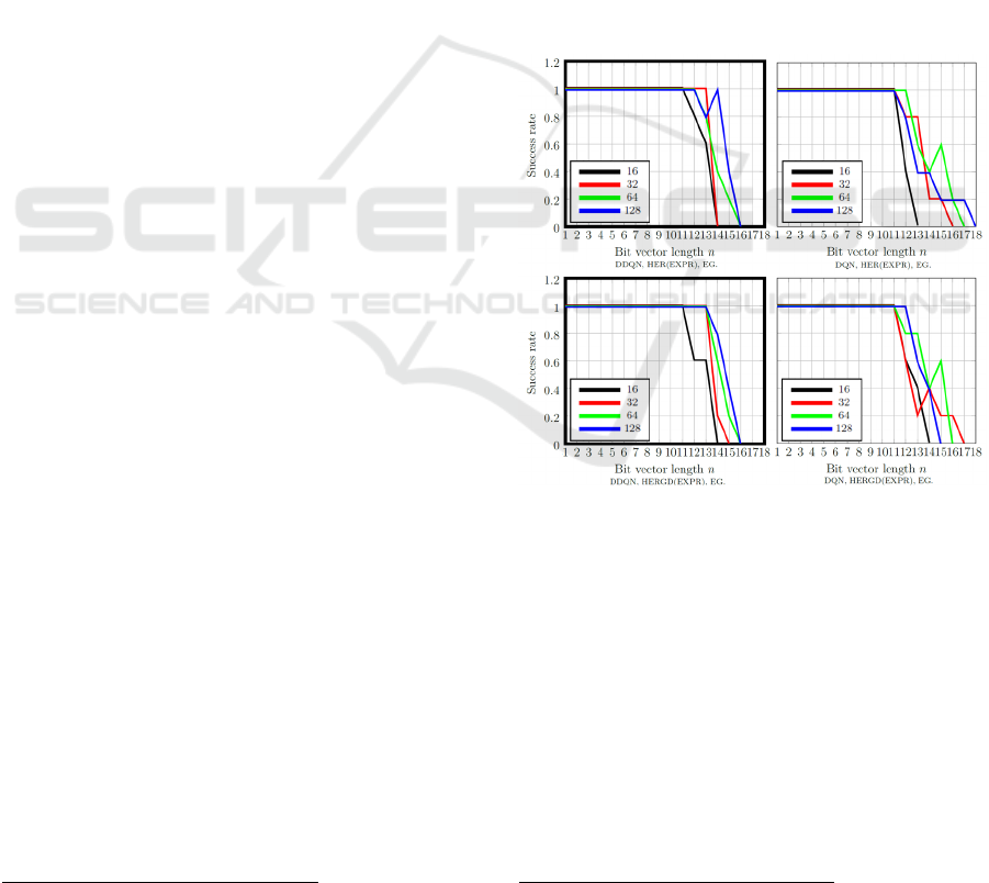
Figure 3 shows representative results of the non-

shaped reward function. With raising bit vector

lengths, the target bit vector 



is more

challenging to discover. Only HER has the advantage

that the Q-network knows the goal state of the

environment right from the beginning. HERGD first

has the same discovery issue as PPROP and EXPR

until the goal is experienced once. In general, larger

batch sizes in combination with HER, HERGD or

PPROP helps when dealing with sparse rewards.

Between the batch size 16 and 128, only a difference

of 3 bits was measured, i.e. 21% better results.

Figure 3: Bit-flip environment with non-shaped rewards for

different batch sizes and combinations of Q-Learning,

replay memories and exploration methods.

In the comparison of DQN with DDQN, it can be

observed that DDQN solves a bit vector length n more

consistently, even with smaller batch size like 16.

One reason that DDQN behaved in this evaluation

pretty much like DQN is the low number of episodes

and bit flips to solve for a bit vector length n. Since

the target network used by DDQN is updated slowly

to avoid divergence, this method requires more

training steps than DQN. For DDGP, the environment

was even more challenging to solve because a

https://www.tensorflow.org

ICAART 2020 - 12th International Conference on Agents and Artiﬁcial Intelligence

continuous action space has to be searched, while

DQN and DDQN only have to search a discrete action

space.

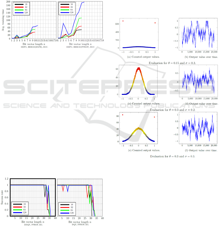
The average training time increases with larger

batch sizes. Also, methods using PPROP or DDPG

require a lot more training time as depicted in

Figure 4. One reason is that the DDPG Q-network

architecture is more complex than the others because

it consists of four neural networks. PPROP internally

uses a sum-tree to store transitions, which increases

training durations.

Figure 4: Training time in the bit-flip environment of

PPROP with non-shaped rewards

The evaluation results of the bit-flip environment

with a shaped reward function can be observed in a

subset of representative results in Figure 5. It can be

noticed that DQN and DDQN were able to solve a

much larger number of bit vector lengths. Reward

shaping drastically improved performance. Only

DDPG performed worse with non-shaped rewards,

which was expected as DDPG is designed for

continuous spaces.

Comparing DQN with DDQN as in Figure 5,

shows that DDQN solves the same bit vector length

more consistently, even with smaller batch sizes, as it

was the case with the non-shaped reward function.

HER and HERGD performed similar but worse than

the EXPR or PPROP. This is not surprising since the

HER (Andrychowicz, 2017) performs badly with

shaped rewards. PPROP performed a little bit better

than EXPR. Average training times do not differ

much from the non-shaped ones.

Figure 5: Success rates in the bit-flip environment of

PPROP with shaped rewards.

5.3.2 Ornstein-Uhlenbeck Process

Parameter Evaluation

In this section, different parameter settings for an OU

and the introduced OUA process are evaluated to

determine which values are useful in certain

environments. All Q-networks use an output range of

1    1. An OU process consists of four

parameters to adjust: θ, σ, μ and a. μ, the mean value

and the starting value are set to 0.0. θ indicates how

fast the process reverts towards the mean. σ

determines the maximum volatility. The evaluation

only records the noise generated by the OU or OUA

process.

Figure 6: The Ornstein-Uhlenbeck process.

Figure 6 shows the evaluation of the standard OU

process with different settings for θ and σ. In the top

graph (θ = 0.15, σ = 0.3), it can be observed that

setting θ < σ will cause the process to output many

values near to the range boundaries. It can be useful

for agents where abrupt control of the actuators is

required. For instance, if a robotic arm is used to

control a heavy mass object, abrupt controlling can be

useful. If θ > σ like in the middle graph, it results in

many output values being close to zero. For agents,

where fine steering is necessary, this setting is useful.

If θ = σ like in the bottom graph, the output values are

Evaluation of Reinforcement Learning Methods for a Self-learning System

concentrated close to zero and at the boundaries of the

range. This setting might be useful for environments

where the entire output range must be covered.

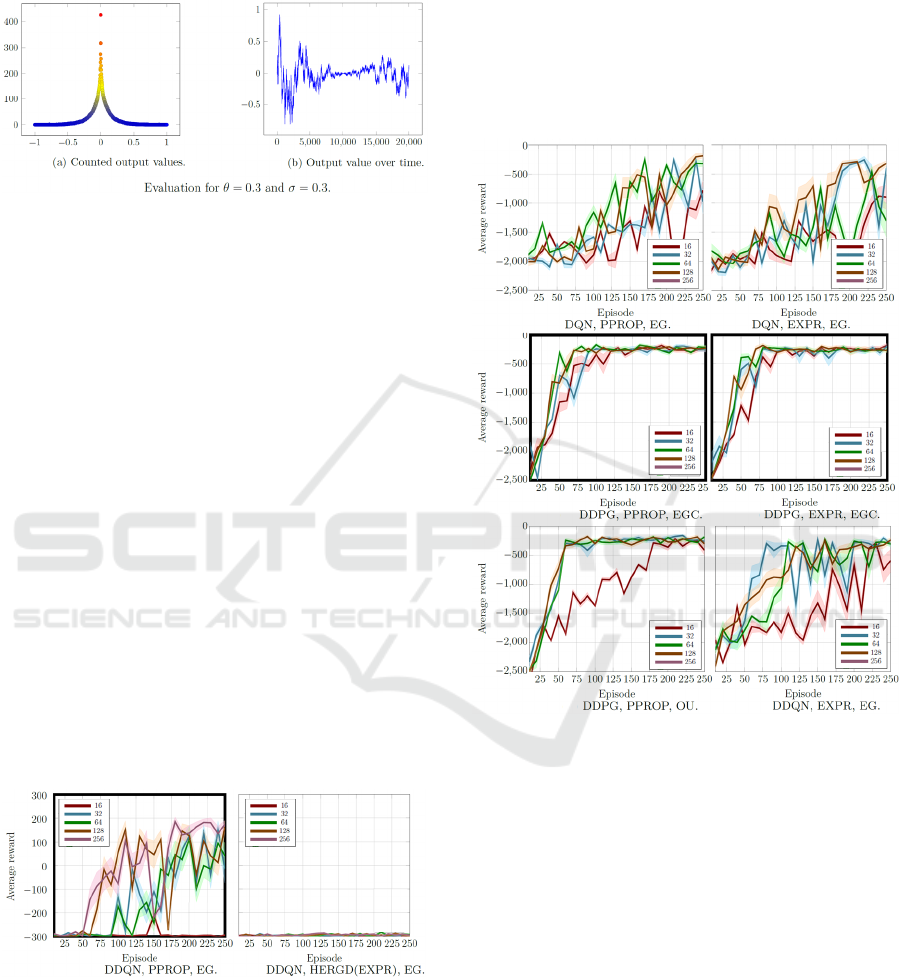
Figure 7: The Ornstein-Uhlenbeck Annealed process.

Results of the introduced OUA process is shown

in Figure 7. Linear decreasing can be observed.

Unfortunately, since an OU process uses the previous

outputted value, the output value increases over some

time again. This behavior is contra-productive, since

it was planned to decrease the outputted noise slowly

to enable soft-switching from exploring to exploiting.

Therefore, the OUA process did not improve the

standard OU method.

5.3.3 Continuous Pendulum Environment

Each tested method has exactly 250 episodes to solve

the pendulum environment. Each episode consists of

300 steps. At each step, an action is predicted by the

Q-network and applied as torque to the pendulum.

After every 10

episode, the learning success is

tested. For this purpose, the learned policy is used

over 20 episodes, and the received rewards are

summed up. Then the mean value is calculated from

the sum of rewards. Also, the standard deviation is

computed and presented as a transparent background

in the graph.

Figure 8: pendulum environment with non-shaped rewards.

The evaluation results of the non-shaped reward

function can be observed in Figure 8. In general, it

can be concluded that the task solving performance is

quite bad. Only, DDQN and DDPG in combination

with EXPR or PPROP as replay memories and EG or

EGC as exploration method managed to perform

acceptably. HERGD was not able to solve the

environment at all. HER delivers quite the same result

as HERGD. In continuous state space environments,

the main goal can only be defined within a small

range. In addition, since the state of the pendulum

environment consists of the vertical velocity, goal

discovery is very bad since the goal is discovered with

a non-zero velocity. This is a limit because the goal is

to keep the pendulum upright in a vertical position.

Figure 9: pendulum environment with shaped rewards.

The evaluation results for the shaped reward

function can be observed in Figure 9. Since HER and

HERGD in combination with shaped reward

functions are documented to perform poorly with

shaped rewards, these evaluations are discarded.

DDPG performed well, while DQN and DDQN did

very poorly in comparison.

Surprisingly, EXPR delivered a little bit better

results than PPROP. Concerning the fact that the

dimension of a discrete state space is countable, this

is not the case for a continuous state space. PPROP

prioritizes the transitions that are new or surprising.

For continuous state spaces, this almost applies to

every transition. Especially this affects the learning

performance for small batch sizes.

For the exploration methods, EGC performed

better than OU, because the behavior of OU is drift-

ICAART 2020 - 12th International Conference on Agents and Artiﬁcial Intelligence

like. In the pendulum environment, it is better to

switch the torque repeatedly from positive to negative

values. This behavior increases the speed and allows

the pendulum to move to a vertical position. Finally,

it results show that PPROP increases the training

times drastically.

5.3.4 Discussion

Based on the evaluations done with the bit-flip

environment and pendulum environment, the best

combinations of the reinforced learning methods are

summarized in Table 1.

For discrete action spaces, it is recommended to

use the Double Deep Q-learning network (DDQN), as

it works better in such environments than the Deep Q-

learning network (DQN) and Deep Deterministic

Policy Gradient (DDPG). On the other side, DDPG

works best for continuous action spaces.

If continuous state spaces are considered, it is

recommended to use Experience Replay (EXPR) as

replay memory, because it performs quite the same as

Proportional Based Prioritized Experience Replay

(PPROP) and HERGD, but requires less training

time. On the other hand, for discrete state space

environments, where a non-shaped reward function is

used, it is recommended to use Hindsight Experience

Replay With Goal Discovery (HERGD) in

combination with PPROP. This will help to

successfully solve sparse reward environments.

Regarding the batch size, it is recommended to

choose a larger value depending on how sparse the

rewards are. The selection of the exploration method

has to be tuned based on the environment. In all cases,

a shaped reward function should be used, since it

drastically improves learning performance.

In a real world, robotic environment where the

agent is a robotic arm, standard OU process is

recommended. In environments, such as the

pendulum environment, where drift-like behavior of

the output values is not good, the introduced EGC

performed the best. With the aid of these evaluations,

it is possible to determine which methods should be

used for a robot in continuous action and state space.

5.3.5 Future Improvements

Some issues can be addressed that emerged during

this work. One problem with sparse reward tasks is

that a transition with a positive reward has to be

sampled from replay memory and has to be

propagated back by repeatedly sampling the

predecessor states. The Q-network slowly learns

which actions to perform from certain states in order

to reach the rewarding state. If the rewarding state is

perceived only a few times, this process is disturbed.

Considering catastrophic forgetting, successful

learning of the task becomes unlikely. To accelerate

the back propagating of Q-values, the Q-function

could be applied to the transitions before saving an

episode to the replay memory.

In that case, a positive reward is present

throughout an entire episode. Sampling a transition

with positive reward would become more likely. A

disadvantage is that the algorithm would convert

more slowly to the ideal policy. This approach can be

combined with the n-step loss mentioned in

(Vecerik, 2017), which should help to propagate the

Q-values along the trajectories.

A great influence on the learning time and the

learning success would be the improvement of the

exploration methods. Only random exploration

methods are possible because the agent should know

as little as possible about the environment. If there is

a memory limitation like in embedded systems,

count-based exploration methods are not applicable.

Count-based methods that store a counter, how many

times a state has been visited, and what actions are

taken to exit the state (Tang, 2016). Instead of

applying noise only to the output neurons, it could be

applied to the entire Q-network (Plappert, 2017).

Table 1: Summary of the best reinforced learning method combinations based on reward function.

Reward function

Non shaped shaped

cont. action space

cont. state space

DDPG, EXPR DDPG, EXPR

dis. action space

cont. state space

DDQN, EXPR DDQN, EXPR

cont. action space

dis. state space

DDPG, HERGD(PPROP) DDPG, EXPR

dis. action space

dis. state space

DDQN, HERGD(PPROP) DDQN, PPROP

Evaluation of Reinforcement Learning Methods for a Self-learning System

Another approach is to let the decision maker

adaptively learn the exploration policy in DDPG (Xu,

2018). The advantage is that this approach is scalable

and yields to a better global exploration. The

disadvantage is that this approach consumes more

memory than OU or EGC.

Finally, deep reinforcement learning in

continuous state and time spaces is still not robust to

small environmental changes and hyper parameter

optimization. For DDPG, the effect of every

individual action vanishes if the discretization

timestep becomes infinitesimal (Tallec, 2019). For

the pendulum environment, algorithm parameters

could be tuned to generate better performance

through a continuous-time analysis.

6 CONCLUSION

The main objective of this paper was to analyze which

combinations of reinforcement learning algorithms,

exploration methods and replay memories are most

suitable for discrete and continuous state spaces as

well as action spaces. Tests were performed in a

simulated discrete bit-flip and continuous pendulum

environment.

This research introduced new techniques to the

state-of-the-art methods, such as Hindsight

Experience Replay with Goal Discovery (HERGD),

ε-greedy Continuous (EGC), and Ornstein-

Uhlenbeck Annealed (OUA). While Ornstein-

Uhlenbeck Annealed did not improve performance,

Hindsight Experience Replay with Goal Discovery, ε-

greedy Continuous proved to perform well.

Equipped with a suitable combination of

algorithms, the next step is to transfer it into a self-

learning robot, which is based on embedded

hardware. The robot is supposed to start without

knowing anything about its sensors, actuators and

environment and gradually learn to survive. In

embedded hardware resource constraints will be an

important challenge to handle.

Enabling robots to learn complex tasks through

experience allows us to take a big step into the future.

The applications for such self-learning robots are

limitless. Writing complex algorithms to control

these robots is eliminated because they learn to

control themselves. In addition, through repetition,

they are able to optimize their behavior. Changes in

the environment do not affect them because they can

adapt to them automatically.

ACKNOWLEDGEMENTS

We gratefully acknowledge the financial support

provided to us by the BMVIT and FFG (Austrian

Research Promotion Agency) program Production of

the Future in the SAVE project (864883).

REFERENCES

Andrychowicz, M., Wolski, F., Ray, A., Schneider, J.,

Fong, R., Welinder, P., McGrew, B., Tobin, J., Abbeel,

P., Zaremba, W.: Hindsight Experience Replay. In:

CoRR abs/1707.01495 (2017)

Dayan, P.: The Convergence of TD(lambda) for General

lambda. In: Machine Learning 8 (1992), May, Nr. 3, S.

341–362. – ISSN 1573–0565

van Hasselt, H., Guez, A., S., David: Deep Reinforcement

Learning with Double Q-learning. In: CoRR

abs/1509.06461 (2015)

Hwangbo, J., Sa, I., Siegwart, R., Hutter, M.: Control of a

Quadrotor With Reinforcement Learning. In: IEEE

Robotics and Automation Letters 2 (2017), Oct, Nr. 4,

S. 2096–2103. – ISSN 2377–3766

Kingma, D. P., Ba, J.: Adam: A Method for Stochastic

Optimization. In: CoRR abs/1412.6980 (2014)

Kirkpatrick, J., Pascanu, R., Rabinowitz, N., Veness, J.,

Desjardins, G., Rusu, A. A., Milan, K., Quan, J.,

Ramalho, T., Grabska-Barwinska, A., Hassabis, D.,

Clopath, C., Kumaran, D., Hadsell, R.: Overcoming

catastrophic forgetting in neural networks. In:

Proceedings of the National Academy of Sciences 114

(2017), Nr. 13, S. 3521–3526. – ISSN 0027–8424

Kober, J., Peters, J.: Reinforcement Learning in Robotics:

A Survey. Bd. 12. Berlin, Germany: Springer, 2012, S.

579–610

Lillicrap, T. P., Hunt, J. J., Pritzel, A., Heess, N., Erez, T.,

Tassa, Y., Silver, D., Wierstra, D.: Continuous control

with deep reinforcement learning. In: CoRR

abs/1509.02971 (2015)

Leuenberger G. and Wiering M. (2018). Actor-Critic

Reinforcement Learning with Neural Networks in

Continuous Games.In Proceedings of the 10th

International Conference on Agents and Artificial

Intelligence - Volume 2: ICAART, ISBN 978-989-758-

275-2, pages 53-60. DOI: 10.5220/0006556500530060

Mnih, V., Kavukcuoglu, K., Silver, D., Graves, A.,

Antonoglou, I., Wierstra, D., Riedmiller, M A.: Playing

Atari with Deep Reinforcement Learning. In: CoRR

abs/1312.5602 (2013)

Mnih, V., Kavukcuoglu, K., Silver, D., Rusu, A., Veness,

J., Bellemare, M. G., Graves, A., Riedmiller, M.,

Fidjeland, A. K., Ostrovski, G., Petersen, S., Beattie, C.,

Sadik, A., Antonoglou, I., King, H., Kumaran, D.,

Wierstra, D., Legg, S., Hassabis, D.: Human-level

control through deep reinforcement learning. In: Nature

518 (2015), Februar, Nr. 7540, S. 529–533. – ISSN

00280836

ICAART 2020 - 12th International Conference on Agents and Artiﬁcial Intelligence

Plappert, M., Houthooft, R., Dhariwal, P., Sidor, S., Chen,

R. Y., Chen, X., Asfour, T., Abbeel, P., Andrychowicz,

M.: Parameter Space Noise for Exploration. In: CoRR

abs/1706.01905 (2017)

Ramachandran, P., Zoph, B., Le, Q. V.: Searching for

Activation Functions. In: CoRR abs/1710.05941 (2017)

Schaul, T., Quan, J., Antonoglou, I., Silver, D.: Prioritized

Experience Replay. In: CoRR abs/1511.05952 (2015)

Shi, H. ; Lin, Z. ; Hwang, K. ; Yang, S. ; Chen, J.: An

Adaptive Strategy Selection Method With

Reinforcement Learning for Robotic Soccer Games. In:

IEEE Access 6 (2018), S. 8376–8386. – ISSN 2169–

3536

Schulman, J., Levine, S., Moritz, P., Jordan, M., Abbeel, P.:

Trust Region Policy Optimization. In: CoRR

abs/1502.05477 (2015)

Sutton, R. S.; Barto, Andrew G.: Reinforcement Learning:

An Introduction. MIT Press, 1998

Tallec, C., Blier, L., Ollivier, Y.: Making Deep Q-learning

methods robust to time discretization. arXiv preprint

arXiv:1901.09732 (2019).

Tang, H., Houthooft, R., Foote, D., Stooke, A., Chen, X.,

Duan, Y., Schulman, J., Turck, F. D., Abbeel, P.:

Exploration: A Study of Count-Based Exploration for

Deep Reinforcement Learning. In: CoRR

abs/1611.04717 (2016)

Thrun, S. B.: Efficient Exploration in Reinforcement

Learning. Pittsburgh, PA, USA : Carnegie Mellon

University, 1992. – Forschungsbericht

Vecerik, M., Hester, T., Scholz, J., Wang, F., Pietquin, O.,

Piot, B., Heess, N., Rothörl, T., Lampe, T., Riedmiller,

M. A.: Leveraging Demonstrations for Deep

Reinforcement Learning on Robotics Problems with

Sparse Rewards. In: CoRR abs/1707.08817 (2017)

Xu, T., Liu, Q., Zhao, L., Peng, J.: Learning to Explore with

Meta-Policy Gradient. In: CoRR abs/1803.05044

(2018)

Evaluation of Reinforcement Learning Methods for a Self-learning System