Visualization to Assist Interpretation of the Multilevel Paradigm in

Bipartite Graphs

Diego S. Cintra

, Alan Valejo

, Alneu A. Lopes

and Maria Cristina F. Oliveira

Instituto de Ci

encias Matem

aticas e de Computac¸

ao (ICMC),

University of S

ao Paulo (USP), CP 688, S

ao Carlos SP, 13560-970, Brazil

Keywords:

Visualization, Bipartite Graphs, Multilevel Paradigm, Graph Summarization.

Abstract:

Multilevel methods refer to a general framework for solving optimization problems in large graphs consider-

ing a hierarchy of contracted representations of the target graph. A recent extension to bipartite graphs has

been introduced and successfully employed in diverse applications, but experience suggests the method is

highly susceptible to the choice of vertex matching strategy for graph contraction and on whether the super-

vertices are relevant generalizations to the problem addressed. Although the ﬂexibility in obtaining contracted

representations of an original graph is a potential advantage, appropriate choice and parameterization of the

contracting algorithms is challenging. Experts would beneﬁt from solutions capable of assisting them in as-

sessing alternatives and making informed decisions. In this work we describe a visualization system that

creates an interactive graphical representation of a multilevel graph hierarchy obtained as a result of executing

a multilevel method on bipartite graphs. We provide illustrative case studies showing the proposed visualiza-

tion can support algorithm developers in inspecting and interpreting how different parameter choices in the

coarsening stage impact the resulting multilevel hierarchies.

1 INTRODUCTION

Multilevel methods provide a framework for solv-

ing optimization problems in large graphs (Walshaw,

2004). They gradually reduce a large scale graph by

coarsening it into a hierarchy of successively smaller

graphs; employ a target algorithm to solve the prob-

lem in the smallest graph instance and project the so-

lution thus obtained backwards into the hierarchy of

increasingly complex graph models, up to the original

one. An approximate solution may be thus obtained

in situations where executing the target algorithm di-

rectly on the original graph might be unfeasible. This

general framework has been instantiated in a variety

of combinatorial problems in graphs, e.g., sparse ma-

trix factorization (Gupta et al., 1997), graph partition-

ing (Padmavathi and George, 2014) and graph draw-

ing (Hachul and J

unger, 2004). Solving a problem on

a small graph requires searching a reduced solution

space rather than the possibly cost-prohibitive solu-

tion space associated with the full graph. Thus, a so-

lution is computed at a reduced cost and then gener-

https://orcid.org/0000-0002-7278-0611

https://orcid.org/0000-0002-9046-9499

https://orcid.org/0000-0003-3112-4746

https://orcid.org/0000-0002-4729-5104

alized to the original graph. The quality of the ﬁnal

solution depends both on the quality of the initial so-

lution and the generalization capability of the graph

contraction strategy.

Originally deﬁned on homogeneous networks, in

which the vertices represent entities of a single type,

the multilevel approach has recently been extended to

bipartite graphs and networks (Valejo et al., 2018).

Vertices in bipartite graphs represent two types of

entities, so that the vertex set is split into two non-

overlapping subsets and edges can only connect ver-

tices in different subsets. Such graphs occur fre-

quently in data analysis scenarios, e.g., document-

word and protein-ligand networks are two illustrative

examples in connection with relevant real-world prob-

lems (Rossi et al., 2016; Jeong et al., 2000).

The framework introduced by Valejo et al. (2018)

to support the multilevel approach on bipartite graphs

is powerful, conceptually simple and highly ﬂexible,

with potential applicability in a wide variety of data

analysis problems. Yet, successful application of mul-

tilevel strategies involves difﬁcult choices, e.g., the

choice and parameterization of vertex matching al-

gorithm required for coarsening may strongly impact

the method’s performance and solution quality. Mak-

ing informed choices when handling novel applica-

Cintra, D., Valejo, A., Lopes, A. and Oliveira, M.

Visualization to Assist Interpretation of the Multilevel Paradigm in Bipar tite Graphs.

DOI: 10.5220/0008903501330140

In Proceedings of the 15th International Joint Conference on Computer Vision, Imaging and Computer Graphics Theory and Applications (VISIGRAPP 2020) - Volume 3: IVAPP, pages

133-140

ISBN: 978-989-758-402-2; ISSN: 2184-4321

133

tion problems is particularly challenging. This work

addresses this gap by introducing a visualization solu-

tion aimed at supporting algorithm developers in in-

specting and interpreting the graph hierarchy result-

ing from an execution of the multilevel method on bi-

partite graphs. Our solution relies on a novel graphi-

cal metaphor for depicting a multilevel bipartite graph

hierarchy, which is the key component of an interac-

tive interface implemented as a front-end to the afore-

mentioned framework.

This paper is organized as follows. The multilevel

strategy is detailed in Section 2, and related work is

brieﬂy reviewed in Section 3. In Section 4 we de-

scribe the components of the visualization system de-

veloped and in Section 5 we present case studies illus-

trating how it can support developers interpreting the

behavior of the multilevel method and understanding

the implications of alternative choices. Concluding

remarks are presented in Section 6.

2 MULTILEVEL METHOD ON

BIPARTITE GRAPHS

A graph G = (V, E) is deﬁned by a set of vertices V

and a set of edges E that indicate relationships be-

tween pairs of vertices. The set V in a bipartite graph

G = (V

, V

, E) is split into two disjoint subsets (lay-

ers) V

and V

, V

∩V

0, and edges connect vertices

in different layers (Bondy et al., 1976). Edges or ver-

tices may have weigths or other attributes. Vertices u

and v are neighbors (adjacent) if edge (v, u) ∈ E. The

degree of v ∈ V, d

(v), is equal to the total weight

of its adjacent edges. The vertex h-hop neighborhood

consists of the vertices in set Γ

(v) = {u| there is a

path of length h between v and u} (Valejo et al., 2018).

Figure 1 illustrates the stages of a multilevel

method applied to a bipartite graph. Initially a

coarsening algorithm creates a sequence of simpliﬁed

(coarsened) versions of the input graph at gradually

increasing contraction levels. Coarsening comprises

the steps of matching, which selects which vertices

will be collapsed; and contraction, which builds the

reduced representation, collapsing the matched ver-

tices and their incident edges into so-called super-

vertices and super-edges, respectively. A super-

vertex is called a successor of its originating ver-

tices, which are themselves called predecessors of the

super-vertex. An initial solution to the target problem

is computed on the coarsest graph instance. In the

ﬁnal uncoarsening stage this initial solution is pro-

jected backwards and reﬁned through the intermedi-

ate sequence of coarsened graphs, until obtaining the

ﬁnal solution in the original input graph.

Figure 1: Multilevel method applied to a bipartite graph G

the coarsening stage computes a sequence of intermediate

coarsened graphs {G

, ..., G

S−1

, G

} from G

, wherein G

is the coarsest graph, on which an initial solution to a tar-

get problem is computed. The uncoarsening stage projects

this initial solution backwards onto the intermediate graphs

S−1

, ..., G

} down to G

, yielding the ﬁnal solution.

The vertex matching algorithm is a key component

of an effective multilevel solution. Inadequate match-

ings may yield poor initial solutions, or poor perfor-

mance of the target algorithm, perhaps both. For-

mally, a matching

M = {V

}

k=0

is a partition of V

into a set of K non-empty and disjoint subsets V

∈ V ,

1 ≤ |V

|, ∀i and i 6= j ⇒ V

∩V

= ∅. A vertex u ∈ V

is called matched, otherwise, if @V

∈ M | u ∈ V

, u is

called unmatched. Algorithms rely on a user-provided

function to assess vertex similarity, e.g., Common

Neighbors (Watts, 2004) considers the pair of ver-

tices with more neighbors in common as the most

similar; Adamic Adar (Adamic and Adar, 2003) re-

lies on a logarithm function to deﬁne a “relevance

factor” in assessing vertex similarity; Preferential At-

tachment (Newman, 2001) considers the adjacent ver-

tex of highest degree as the most similar.

Many matching algorithms have been developed

relying on different policies to establish how vertices

will be collapsed. We brieﬂy review two recent al-

gorithms targeted at bipartite graphs, namely GMb

(Greedy Matching for bipartite graphs) (Valejo et al.,

2018) and MLPb (Multilevel Label Propagation for

bipartite graphs) (Valejo et al., 2019a). Both take as

input parameters the initial graph G

; the layers to be

coarsened, i.e., if layer V

, layer V

or both; and the

similarity function S(u, v), u, v ∈ V . Input parameters

are informed with indexes 1 or 2 to indicate they refer

respectively to layer V

or V

GMb matching merges vertices pairwise relying

on a priority queue of candidate pairs v and u, wherein

(v) = u, organized according to their similarity as

computed by the given function S

(u, v), j ∈ 1, 2, so

that highly similar pairs are matched ﬁrst. Addi-

Note, in the mathematical discipline of graph theory, a

matching is deﬁned as a set of independent edges.

IVAPP 2020 - 11th International Conference on Information Visualization Theory and Applications

134

tional inputs are the number of coarsening levels l

and the graph reduction factors r f

. For instance, set-

ting l

= l

= 3 and r f

= r f

= 0.3 creates a 3-level

graph hierarchy G

, G

with each graph layer at a

level k having 30% of its vertices paired into super-

vertices, relative to the previous level k − 1. A max-

imum reduction factor of 50% is attained in a single

iteration. Coarsening large graphs will require many

iterations, incurring in high processing and memory

costs. Moreover, matching quality tends to degrade

towards the ﬁnal iterations, as vertices considered for

matching later are less likely to ﬁnd good candidate

pairs.

MLPb (Multilevel Label Propagation for bipartite

graphs) has been introduced to overcome these limita-

tions. It relies on label propagation to collapse vertex

groups, rather than pairs. Every vertex is initially as-

signed a unique label. At each iteration, each vertex

updates its label with the the most frequent label in its

neighboring vertices. Intuitively, a densely connected

group of vertices will converge to a single dominant

label, and upon convergence vertices with the same

label will be collapsed into a single super-vertex. Be-

sides G

and S

(u, v), MLPb takes as input parame-

ters the desired layer sizes in the coarsest graph, ζ

and a maximum number of iterations T . E.g., given

with |V

| = |V

| = 200, |E| = 10.000 and setting

= ζ

= 20 MLPb will attempt to execute T iter-

ations to create G

with |V

| = |V

| = 20. If this is

not feasible, it will coarsen G

to yield a new graph

and again execute up to T iterations. The pro-

cess continues until the target sizes are met, yielding

a multilevel graph hierarchy.

The bipartite multilevel framework MOb (Valejo

et al., 2018) has been developed in Python as a ﬂex-

ible solution that admits plugging alternative match-

ing algorithms and can be instantiated to solve mul-

tiple categories of problems. It provides the back-

end to our multilevel visualization front-end, called

MObViewer. The aim is to facilitate interpretation of

the behavior and limitations of matching algorithms

and the impact of parameter choices on the outcome

of a multilevel process applied to a bipartite network.

3 RELATED WORK

Multilevel methods have been applied, for instance, to

reduce the computational cost of computing node-link

layouts (Harel and Koren, 2000; Gajer and Kobourov,

2001; Hachul and J

unger, 2004), and an experimental

evaluation of their usage in association with energy-

based layout algorithms has been reported (Bartel

et al., 2011).

Wong et al. (2009) describe a visualization solu-

tion which relies on the hierarchy of coarsened graphs

displayed in interactive node-link views, which users

can browse when executing analysis tasks. Providing

graph views at varying coarsening levels addresses

the visual clutter typical of node-link layouts. In-

deed, whilst node-link representations are intuitive

to convey global topological structures (Ghoniem

et al., 2004), rendering large graphs is computa-

tionally expensive and may yield highly cluttered

views on which exploratory tasks can be severely im-

paired (Von Landesberger et al., 2011).

Visual aggregation of nodes and edges is often

employed to mitigate clutter. Edge bundling is possi-

bly the best established solution for implicit edge ag-

gregation (Lhuillier et al., 2017), whereas vertex ag-

gregation strategies are usually explicit and domain-

driven. Most solutions rely on clustering or com-

munity detection to group vertices into meta-vertices,

super-vertices, clusters or communities (Von Landes-

berger et al., 2011), resulting in a hierarchical repre-

sentation useful for visualization purposes.

Another category of related work comprises re-

cent solutions for exploratory visualization of data

modeled as large scale bipartite graphs. Several

systems employ the biclustering algorithm (Heinrich

et al., 2011) to generate vertex aggregations in this

context (Zhao et al., 2018; Xu et al., 2016; Steinbock

et al., 2018). Yet, other approaches are possible, e.g,

the system WAOW-Vis (Pezzotti et al., 2018) adopts

a hierarchical dimensionality reduction technique to

create hierarchical representations of bipartite graphs

and users may interact to expand a particular region.

The previous contributions deal with issues re-

lated to visualization of large graphs, focusing mostly

on supporting data analysis. Our contribution is dif-

ferent in two ways. First, we deal with the problem of

depicting a hierarchy of graphs resulting from coars-

ening in the context of the multilevel method. Second,

we aim at assisting developers of multilevel solutions

in assessing the effect of distinct choices of coarsen-

ing strategy. We are not aware of previous efforts of

developing interactive visualizations to improve inter-

pretation of the multilevel method or to support navi-

gation in multilevel graph hierarchies, for the case of

either homogeneous or bipartite graphs. Our goal is

to investigate to which extent a visualization of the

multilevel graph hierarchy can enhance user interpre-

tation of the graph generalization process yielded by

the multilevel method, in the particular case of bipar-

tite graphs.

Visualization to Assist Interpretation of the Multilevel Paradigm in Bipartite Graphs

135

4 MObViewer

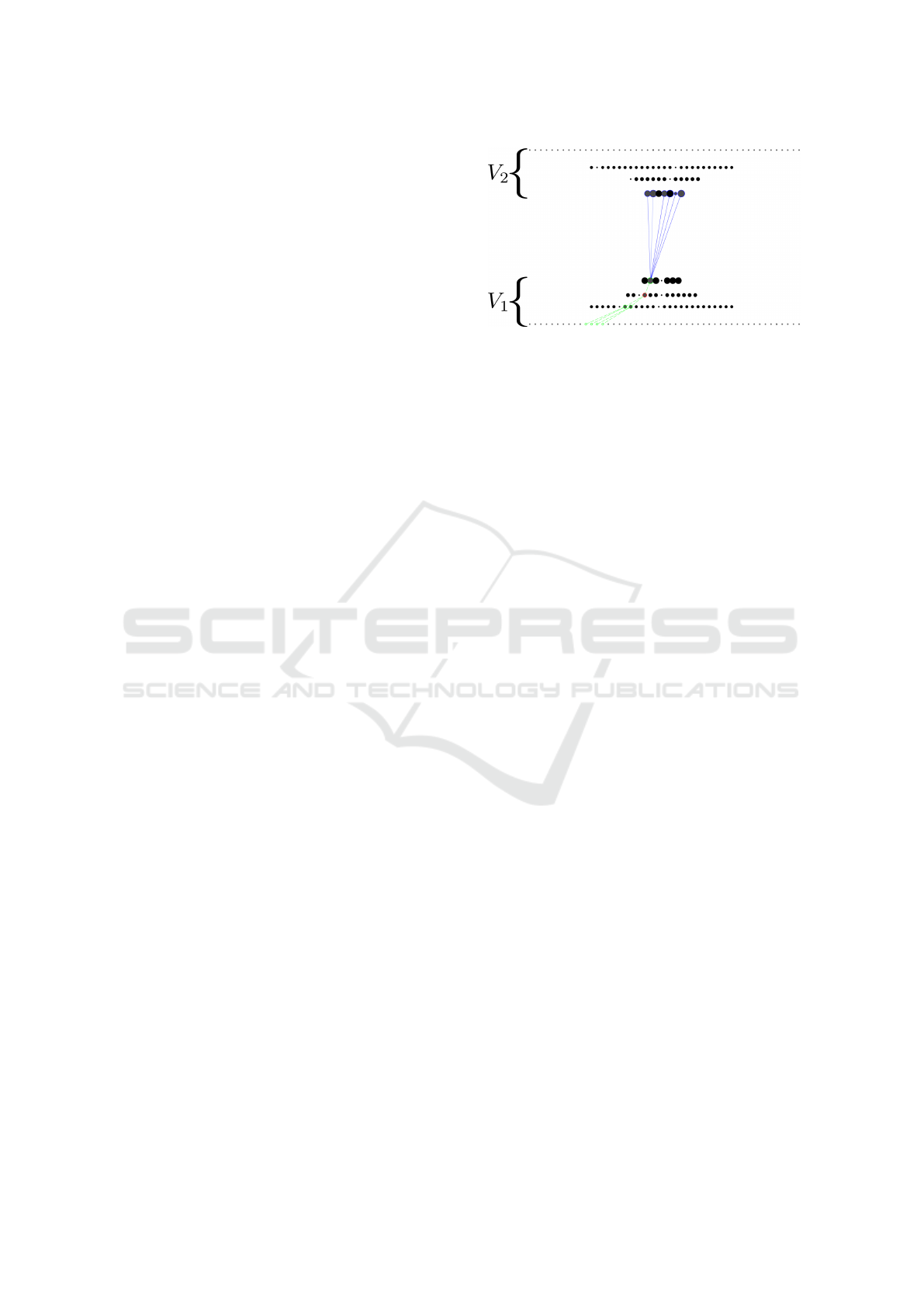
Figure 2 shows MObViewer’s graphical metaphor for

a multilevel graph with four hierarchical levels, where

a vertex has been user selected (outlined in red). Ver-

tices and super-vertices are shown metaphor as circles

of varying sizes, with circle size proportional to the

number of predecessors of the super-vertex. The two

innermost circle rows depict the layers of the coarsest

graph, while moving outwards from the central rows,

the outer rows represent the remaining hierarchy of

intermediate levels for each layer. The two outermost

rows, rendered in gray, depict the layers of the input

graph. By convention, the hierarchy relative to layer

is displayed in the bottom area, whereas the hier-

archy relative to layer V

is shown at the top.

Edges are rendered on-demand, upon vertice se-

lection: once the user selects a vertex its correspond-

ing circle is outlined in red and its incident edges

are rendered. This choice has the beneﬁt of avoiding

line clutter and overdrawing. There are two types of

edges: adjacency edges, rendered in blue as full lines,

and hierarchy edges, rendered as green dotted lines.

The ﬁrst deﬁne the actual graph topology, i.e., how

vertices in layers V

and V

are connected. The second

show a vertex connections to their successor or pre-

decessor (super-)vertices in the multilevel hierarchy.

Adjacency edges are only displayed at the coarsest

graph level, i.e., between the two inner rows/layers.

Since graph layers are stacked on top/bottom of each

other, the vertices are lined-up placing all predeces-

sors of a super-vertex side-by-side, which prevents

edge crossing and allows users to easily track which

vertices have been grouped into a super-vertex. The

complete thread of edges connecting a selected vertex

to its predecessor/successor vertices is shown, with

the circles depicting vertices in the hierarchical path

outlined in green; and the circles depicting the adja-

cent vertices to the selected one outlined in blue. For

weighted graphs the weights of adjacency edges are

mapped to color intensity, so darker shades of blue

indicate heavier edges.

MObViewer has been implemented as a client-

server web application, with the back-end running

MOb and the front-end running the visualization mod-

ule. We used Javascript for implementation, with

Node.js on the server-side; Express.js, a middleware

for server-client data routing and communication;

Three.js to render the graph metaphor and D3.js (Bo-

stock et al., 2011) functions for visualization. MOb-

Viewer is available to interested readers at https:

//github.com/diego2337/MObViewer.

Figure 2: Visual metaphor depicting a multilevel graph hi-

erarchy, with a selected vertex (outlined in red) and its adja-

cency edges (blue lines) and hierarchy edges (green lines).

5 RESULTS

We illustrate how MObViewer can support developers

of multilevel solutions. The software has been exe-

cuted on a Linux Mint 18.2 with 32GB RAM, Intel

Core i7-3770 3.40 GHz and video card GeForce GTX

660. We considered scenarios of interest to develop-

ers of multilevel solutions, and report results from an

empirical investigation of the following questions rep-

resentative of issues faced by users of matching and

coarsening algorithms:

Q1 How does the choice of similarity function af-

fect preservation of the community structures in

the multilevel hierarchy?

Q2 Is it possible to identify at which point in coars-

ening community structures start to degrade, i.e.,

super-vertices are created with predecessors ver-

tices from multiple communities?

Q3 How does parameter reduction factor impact the

construction of the multilevel hierarchy?

Q4 Is the matching algorithms’ capability of preserv-

ing community structures affected by the number

of communities in the input graph?

MobViewer allows inspecting how the match-

ing algorithms behave with distinct parameter set-

tings, and thereby comparing the outcome of differ-

ent choices and assessing the convenience of adopt-

ing alternative strategies. Indeed, the ability to ‘see’

a multilevel graph hierarchy and its properties is an

important facility for developers. Here we present

illustrative scenarios of how each question could be

investigated, taking as example a particular combina-

tion of algorithm, parameter settings and input graph.

Of course, these questions are just a sample of what

might be asked and they could be further investigated

considering other settings.

In order to study the method’s behavior on graphs

with diverse properties we synthesized weighted bi-

IVAPP 2020 - 11th International Conference on Information Visualization Theory and Applications

136

partite graphs with arbitrary community structures

and topological properties using a benchmarking

tool called BNOC (Benchmarking weighted Bipar-

tite Networks with Overlapping Community struc-

ture) (Valejo et al., 2019b). Table 1 summarizes the

synthetic networks considered. Graphs SG

and SG

are sparse with an equal number of communities in

both layers, whereas graph SG

is denser with 3 com-

munities in layer V

and 5 in layer V

. Graphs SG

and SG

have vertex sets of the same size, but SG

denser and the graphs differ in the number of commu-

nities in each layer.

Table 1: Synthetic graphs used in case studies.

Graph Vertices Edges V

Communities

100 555 50 50 [4, 4]

1.000 6.603 500 500 [7, 7]

1.819 23.052 542 1.277 [3, 5]

15.000 189.254 10.000 5.000 [15, 15]

15.000 19.102 10.000 5.000 [40, 40]

In order to answer questions Q1 and Q2 we con-

sidered three conﬁgurations of the multilevel method

using GMb matching with distinct similarity func-

tions: “Common Neighbors” in conﬁguration C.CN,

“Adamic Adar” in C.AA and “Preferential Attach-

ment” in C.PA. In the ﬁgures, glyph colors map the

corresponding vertex communities; glyphs represent-

ing super-vertices may have multiple colors reﬂecting

the community distribution of their predecessors.

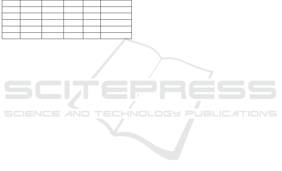
Figure 3 shows the hierarchy of coarsened graphs

obtained executing MOb on SG

with the three con-

ﬁgurations. The hierarchy yielded by conﬁguration

C.CN, Figure 3(a), includes a few super-vertices with

predecessors from mixed communities, outlined in

red. Conﬁguration C.PA, Figure 3(c), did not pre-

serve the community structure, which was best pre-

served with the settings of conﬁguration C.AA, Fig-

ure 3(b). Equivalent analyses were conducted on SG

and SG

(not shown), with similar conclusions.

Addressing related question Q2, Figures 4(a)

and 4(b) show two closer views of the multilevel hier-

archies of graph SG

yielded by conﬁgurations C.PA

and C.CN, respectively. In the multilevel graph in

Figure 4(a) one notices vertices from distinct commu-

nities merging into a single super-vertex at the second

hierarchical level, see the zoomed-in views. However,

in the multilevel hierarchy computed with conﬁgura-

tion C.CN, shown in Figure 4(b), super-vertices with

mixed communities only appear at the ﬁnal levels.

Community structure was best preserved with Com-

mon Neighbors similarity, Figure 4(b).

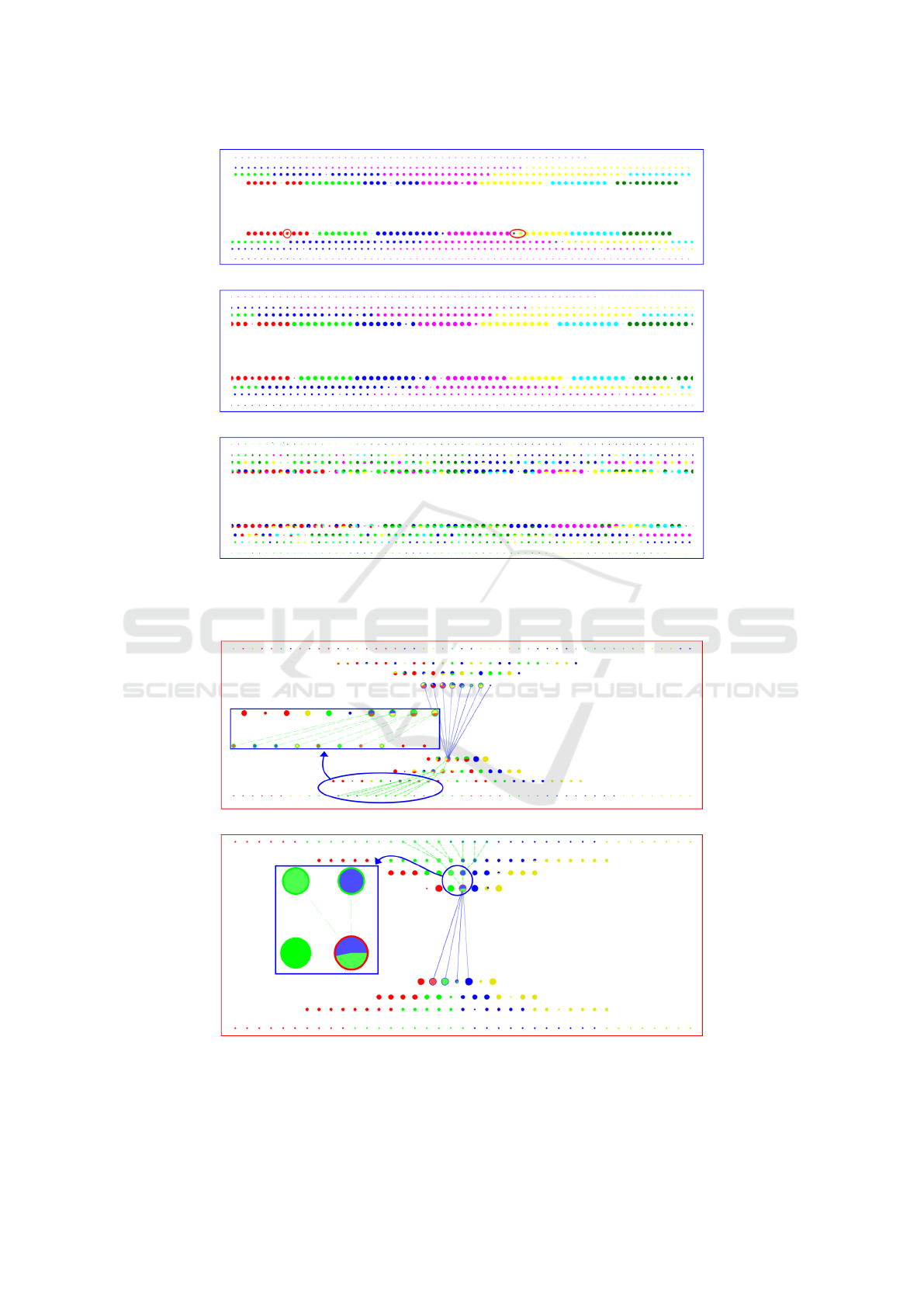
In order to address question Q3 we executed the

multilevel method again with the GMb matching algo-

rithm and the “Common Neighbors” similarity, with

4 distinct settings of parameters reduction factor and

number of levels (applied to both layers), informed

in Figure 5, which shows the corresponding coarsest

graphs SG

. The number of super-vertices is strongly

affected by the choice of r f , i.e., as reduction factors

decrease fewer super-vertices are created and they are

more imbalanced in size; notice, for instance, the

super-vertices in Figures 5(a) and (d). Figure 6 shows

an equivalent analysis on graph SG

considering two

extreme conﬁgurations. Unlike the coarsest graph

in (a), where most super-vertices have predecessors

originating from a single community, the graph in (b)

has just 2 super-vertices (outlined in red) with pre-

decessors from mixed communities. Small reduc-

tion factors imply in few super-vertices, very likely

formed by predecessor vertices from multiple com-

munities, impairing community preservation.

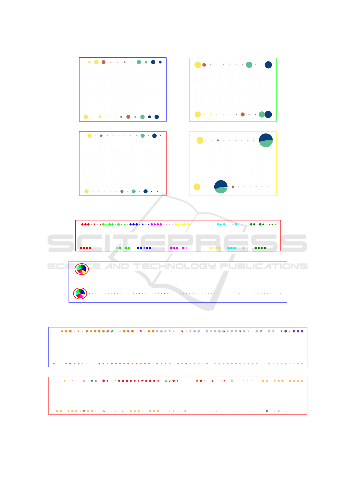
Question Q4 was investigated on SG

, a sparse

graph with 40 communities in each layer, again us-

ing the “Common Neighbors” similarity. We applied

two different matchings, MLPb with ζ

= 3.900, ζ

1.200 and T = 1, and GMb with r f

= r f

= 0.5

and l

= l

= 3 (settings chosen to obtain a coarsest

level graph with layers of equivalent sizes to MLPb).

Figure 7 shows the coarsest level graphs, which for

the most part preserved the community structures in

merging vertices. This example illustrates that both

algorithms, despite adopting very distinct strategies,

can preserve the community structures even in graphs

with many communities. Other conﬁgurations were

investigated, yielding similar results (not shown).

6 CONCLUSIONS

We introduced MObViewer, a visualization tool that

supports interpreting the outcome of executing the

multilevel method on bipartite graphs. It relies on a

visual metaphor designed to depict multilevel bipar-

tite graphs hierarchies computed with the MOb frame-

work. Illustrative case studies conﬁrmed its capabil-

ity of conveying the behavior of a matching algorithm

applied with distinct parameter settings. Thus, devel-

opers of multilevel solutions can quickly assess alter-

native conﬁgurations in order to interpret and under-

stand the impact of choices of matching algorithm,

similarity function, and reduction factors.

Scalability is a critical issue in MObViewer. In

spite of using state-of-the-art technologies the current

implementation does not scale to graphs with roughly

over 20.000 vertices or 30.000 edges. Performance

is also hindered on multilevel hierarchies with many

intermediate coarsening levels. On-demand network

processing could be considered to overcome scalabil-

ity limitations on interactive visual data analytics sce-

Visualization to Assist Interpretation of the Multilevel Paradigm in Bipartite Graphs

137

(a) C.CN{r f

= r f

= 0.5, l

= l

, S =Common Neighbors}

(b) C.AA{r f

= r f

= 0.5, l

= l

, S =Adamic Adar}

= r f

= 0.5, l

= l

, S =Pref. Attachment}

Figure 3: Multilevel hierarchies resulting from coarsening SG

with GMb matching considering 3 distinct similarity functions

S: community structures were best preserved using the Adamic Adar and Common Neighbors functions (a, b).

(a) C.PA{r f

= r f

= 0.5, l

= l

= 3, S =Pref. Attachment}

(b) C.PA{r f

= r f

= 0.5, l

= l

= 3, S =Common Neighbors}

Figure 4: User-selected super-vertex in graph SG

and the thread of edges to its predecessors in 2 multilevel hierarchies

obtained with 2 distinct choices of S. (a) shows super-vertices with predecessors from mixed communities at level 2 of the

hierarchy; in (b) such vertices only appear at the coarsest level (zoomed-in views of the areas outlined in blue are shown).

IVAPP 2020 - 11th International Conference on Information Visualization Theory and Applications

138

(a) C1{r f

= r f

= 0.4, l

= l

= 3} (b) C2{r f

= r f

= 0.3, l

= l

= 5}

= r f

= 0.1, l

= l

= 16} (d) C4{r f

= r f

= 0.2, l

= l

= 7}

Figure 5: Coarsest graphs of the multilevel hierarchies computed for SG

with 4 distinct parameter settings in GMb.

(a) C.1{r f

= r f

= 0.4, l

= l

= 4} S =Common Neighbors.

(b) C.2{r f

= r f

= 0.1, l

= l

= 20} S =Common Neighbors.

Figure 6: Coarsest graphs of the multilevel hierarchy obtained from graph SG

with two settings of GMb.

(a) Coarsest graph from MLPb matching with ζ

= 3.900, ζ

= 1.200, T = 1.

(b) Coarsest graph from GMb matching with r f

= r f

= 0.5 and l

= l

= 3.

Figure 7: Coarsest level graphs after coarsening SG

with different matching algorithms and S =Common Neighbors.

Visualization to Assist Interpretation of the Multilevel Paradigm in Bipartite Graphs

139

narios. Rather than processing the full network in a

batch-like operation mode, the system could build and

process a sub-network reﬂecting a current user focus

on-the-ﬂy, where these sub-networks satisfying a user

requirement would likely have manageable sizes. Ad-

ditional interaction facilities could be incorporated,

such as supporting interaction with selected levels of

the multilevel hierarchy. Further validation on addi-

tional scenarios is also necessary.

ACKNOWLEDGEMENTS

The authors acknowledge the ﬁnancial support of

FAPESP grants 2016/25107-0 and 2017/05838-3 and

CNPq grants 134806/2016-6 and 301847/2017-7.

REFERENCES

Adamic, L. A. and Adar, E. (2003). Friends and neighbors

on the web. Social Networks, pages 211–230.

Bartel, G., Gutwenger, C., Klein, K., and Mutzel, P. (2011).

An experimental evaluation of multilevel layout meth-

ods. In Graph Drawing, pages 80–91, Berlin, Heidel-

berg. Springer.

Bondy, J. A., Murty, U. S. R., et al. (1976). Graph theory

with applications, volume 290. Elsevier Science Ltd.,

Oxford, UK.

Bostock, M., Ogievetsky, V., and Heer, J. (2011). D3:

Data-driven documents. IEEE Trans. Visualization

and Computer Graphics, 17(12):2301–2309.

Gajer, P. and Kobourov, S. G. (2001). Grip: Graph draw-

ing with intelligent placement. In Marks, J., editor,

Graph Drawing, pages 222–228, Berlin, Heidelberg.

Springer Berlin Heidelberg.

Ghoniem, M., Fekete, J. D., and Castagliola, P. (2004). A

comparison of the readability of graphs using node-

link and matrix-based representations. IEEE Symp.

Information Visualization, pages 17–24.

Gupta, A., Karypis, G., and Kumar, V. (1997). Highly scal-

able parallel algorithms for sparse matrix factoriza-

tion. IEEE Trans. Parallel and Distributed Systems,

8(5):502–520.

Hachul, S. and J

unger, M. (2004). Drawing large graphs

with a potential-ﬁeld-based multilevel algorithm. In

Proc. 12th Int. Conf. Graph Drawing, GD’04, pages

285–295, Berlin, Heidelberg. Springer.

Harel, D. and Koren, Y. (2000). A fast multi-scale method

for drawing large graphs. Proc. Working Conf. Ad-

vanced Visual Interfaces, pages 282–285.

Heinrich, J., Seifert, R., Burch, M., and Weiskopf, D.

(2011). Bicluster viewer: A visualization tool for

analyzing gene expression data. In Advances in Vi-

sual Computing, pages 641–652, Berlin, Heidelberg.

Springer Berlin Heidelberg.

Jeong, H., Tombor, B., Albert, R., Oltvai, Z. N., and

Barab

asi, A.-L. (2000). The large-scale organization

of metabolic networks. In Nature, volume 407, page

651. Nature Publishing Group.

Lhuillier, A., Hurter, C., and Telea, A. (2017). State of the

art in edge and trail bundling techniques. Computer

Graphics Forum, pages 619–645.

Newman, M. E. (2001). The structure of scientiﬁc collabo-

ration networks. Proc. National Academy of Sciences,

pages 404–409.

Padmavathi, S. and George, A. (2014). Multilevel hybrid

graph partitioning algorithm. In IEEE Int. Advance

Computing Conf., pages 85–89.

Pezzotti, N., Fekete, J.-D., H

ollt, T., Lelieveldt, B., Eise-

mann, E., and Vilanova, A. (2018). Multiscale vi-

sualization and exploration of large bipartite graphs.

Computer Graphics Forum, pages 12–25.

Rossi, R. G., de Andrade Lopes, A., and Rezende, S. O.

(2016). Optimization and label propagation in bipar-

tite heterogeneous networks to improve transductive

classiﬁcation of texts. Information Processing & Man-

agement, pages 217 – 257.

Steinbock, D., Groller, E., and Waldner, M. (2018). Casual

visual exploration of large bipartite graphs using hier-

archical aggregation and ﬁltering. Int. Symp. Big Data

Visual and Immersive Analytics, pages 1–10.

Valejo, A., Faleiros, T., Oliveira, M. C. F., and Lopes, A. A.

(2019a). A coarsening method for bipartite networks

via weight-constrained label propagation. Knowledge-

Based Systems (accepted).

Valejo, A., G

oes, F., Romanetto, L., Oliveira, M. C. F., and

Lopes, A. A. (2019b). A benchmarking tool for the

generation of bipartite network models with overlap-

ping communities. Knowledge and Information Sys-

tems.

Valejo, A., Oliveira, M. C. F., R. Filho, G. P., and Lopes,

A. A. (2018). Multilevel approach for combinatorial

optimization in bipartite networks. Knowledge-Based

Systems, pages 45–61.

Von Landesberger, T., Kuijper, A., Schreck, T., Kohlham-

mer, J., van Wijk, J. J., Fekete, J.-D., and Fellner,

D. W. (2011). Visual analysis of large graphs: state-

of-the-art and future research challenges. Computer

Graphics Forum, pages 1719–1749.

Walshaw, C. (2004). Multilevel reﬁnement for combina-

torial optimisation problems. Annals of Operations

Research, pages 325–372.

Watts, D. J. (2004). Small worlds: the dynamics of networks

between order and randomness, volume 9. Princeton

University Press.

Wong, P. C., Mackey, P., Cook, K. A., Rohrer, R. M., Foote,

H., and Whiting, M. A. (2009). A multi-level middle-

out cross-zooming approach for large graph analytics.

IEEE Symp. Visual Analytics Science and Technology.,

pages 147–154.

Xu, P., Cao, N., Qu, H., and Stasko, J. (2016). Interactive

visual co-cluster analysis of bipartite graphs. IEEE

Paciﬁc Visualization Symp., pages 32–39.

Zhao, J., Sun, M., Chen, F., and Chiu, P. (2018). Bidots: Vi-

sual exploration of weighted biclusters. IEEE Trans.

Visualization and Computer Graphics, pages 195–

204.

IVAPP 2020 - 11th International Conference on Information Visualization Theory and Applications

140