SSD-ML: Hierarchical Object Classiﬁcation for Trafﬁc Surveillance

M. H. Zwemer

1,2

, R. G. J. Wijnhoven

and P. H. N. de With

Department of Electrical Engineering, Eindhoven University of Technology, Eindhoven, The Netherlands

ViNotion B.V., Eindhoven, The Netherlands

Keywords:

Surveillance Application, SSD Detector, Hierarchical Classiﬁcation.

Abstract:

We propose a novel CNN detection system with hierarchical classiﬁcation for trafﬁc object surveillance. The

detector is based on the Single-Shot multibox Detector (SSD) and inspired by the hierarchical classiﬁcation

used in the YOLO9000 detector. We separate localization and classiﬁcation during training, by introduc-

ing a novel loss term that handles hierarchical classiﬁcation. This allows combining multiple datasets at

different levels of detail with respect to the label deﬁnitions and improves localization performance with

non-overlapping labels. We experiment with this novel trafﬁc object detector and combine the public UA-

DETRAC, MIO-TCD datasets and our newly introduced surveillance dataset with non-overlapping class def-

initions. The proposed SSD-ML detector obtains 96.4% mAP in localization performance, outperforming

default SSD with 5.9%. For this improvement, we additionally introduce a speciﬁc hard-negative mining

method. The effect of incrementally adding more datasets reveals that the best performance is obtained when

training with all datasets combined (we use a separate test set). By adding hierarchical classiﬁcation, the aver-

age classiﬁcation performance increases with 1.4% to 78.6% mAP. This positive result is based on combining

all datasets, although label inconsistencies occur in the additional training data. In addition, the ﬁnal system

can recognize the novel ‘van’ class that is not present in the original training data.

1 INTRODUCTION

Thousands of surveillance cameras are placed along

public roads and highways for trafﬁc management

and law enforcement. Because continuous manual in-

spection is infeasible, only a limited number of cam-

eras are observed, speciﬁcally for special situations

(trafﬁc jams, accidents). Video analysis tools enable

automatic detection of such situations, improving the

efﬁciency of trafﬁc incident management. In addition

to real-time safety management, the output of such

detection, tracking and classiﬁcation algorithms gen-

erate interesting statistics about the amount and type

of road users and their presence over time and on

road lanes. Multi-fold solutions for automatic recog-

nition of road users have been proposed (Sivaraman

and Trivedi, 2013; Fan et al., 2016; Lyu. et al., 2018).

All these works focus on detection and tracking and

apply classiﬁcation only with a limited number of ob-

ject classes.

Depending on the application, a varying amount

of detail is desired in the number of classes. For gen-

eral trafﬁc management, it is sufﬁcient to distinguish

between small trafﬁc (cars, motorcycles) and large

trafﬁc (trucks and buses). In the application of tolling,

a larger number of classes is desired (extra classiﬁca-

tion of agricultural vehicles, and articulated vs. ﬁxed-

unit trucks or even a division in the number of axles).

For law enforcement or predicting CO2 emissions, a

higher classiﬁcation resolution is required, such as ve-

hicle brand, model and engine type/size.

Although vehicle categories can be found by read-

ing the license plate and querying detailed informa-

tion in a national registry, the license plate might not

be visible or readable, due to occlusions or limited

pixel size and lack of database availability. Other

solutions for classiﬁcation comprise expensive laser

scanners that are required to be mounted at exact po-

sitions above the road. A less intrusive and more

maintenance-friendly solution is the use of video

cameras. When considering cameras for monitoring

crossings or busy roads, visual detection and classi-

ﬁcation of vehicles is required because license plates

are too small for automatic plate recognition. Given

these considerations, a detailed visual trafﬁc object

classiﬁcation is indispensable based on video camera

information. However, this classiﬁcation cannot fur-

ther proceed without discussing available datasets.

In recent years, substantial work has been done

on visual object detection and classiﬁcation for which

250

Zwemer, M., Wijnhoven, R. and de With, P.

SSD-ML: Hierarchical Object Classiﬁcation for Trafﬁc Surveillance.

DOI: 10.5220/0008902402500259

In Proceedings of the 15th International Joint Conference on Computer Vision, Imaging and Computer Graphics Theory and Applications (VISIGRAPP 2020) - Volume 5: VISAPP, pages

250-259

ISBN: 978-989-758-402-2; ISSN: 2184-4321

various image vehicle datasets have been published,

such as the UA-DETRAC (Wen et al., 2015) and

MIO-TCD (Luo et al., 2018) datasets. As detection

and classiﬁcation algorithms gained improved perfor-

mance, novel datasets have been labeled in more de-

tail. Because of this continuous growth in detail in

categories between datasets, combining such data re-

quires the alignment of classiﬁcation labels.

In this paper, the global objective is on visual ob-

ject detection and classiﬁcation of vehicle trafﬁc in

surveillance scenarios. For detailing the classiﬁca-

tion, we propose the use of an hierarchical category

deﬁnition, that combines datasets at different levels

of detail in classiﬁcation label deﬁnitions. This is

implemented by adopting an existing Convolutional

Neural Network (CNN) detector for hierarchical clas-

siﬁcation. This detector is trained using datasets la-

beled with different levels of hierarchical labels, com-

bining the classes of multiple datasets. We show

that object classes that are not labeled in one dataset

can be learned from other datasets where these la-

bels do exist, while exploiting other information from

the initial dataset. This allows for incremental and

semi-automatic annotation of datasets with a limited

amount of label detail. As a result of our method, the

obtained classiﬁcation is completely tailored to our

desired hierarchical classiﬁcation, while our method

is ﬂexible to the input data and can accept a broad

range of pre-categorized datasets.

2 RELATED WORK

State-of-the-art object detectors in computer vision

typically perform detection in two stages. In the ﬁrst

stage, they determine if there is an object and in the

second stage they determine its category and regress

the exact location of the object. For example, R-

CNN (Girshick et al., 2014), Fast R-CNN (Girshick,

2015), Faster R-CNN (Ren et al., 2015) and Mask R-

CNN (He et al., 2017) select object proposals in the

ﬁrst stage and then classify and reﬁne the bounding

box in a second stage. The two stages already intro-

duce hierarchy: object vs. background at the top and

the different object categories beneath, but subcate-

gories are not considered. Generally, a disadvantage

of two-stage detectors is that they are more complex

than recent single-stage detectors.

Single-stage detectors perform object localization

and classiﬁcation in a single CNN. The most popu-

lar single-stage detectors are YOLO (Redmon et al.,

2016; Redmon and Farhadi, 2017), SSD (Liu et al.,

2016) and the more recent FCOS (Tian et al., 2019).

The YOLO detector uses the topmost feature map of

a base CNN network to predict bounding boxes di-

rectly for each cell in a ﬁxed grid. The SSD detector

extends this concept by using multiple default bound-

ing boxes with various aspect ratios. In addition, SSD

uses multi-scale versions of the top-most feature map,

rendering the SSD detector more robust to large vari-

ations in object size. Therefore, we propose to use the

SSD detector as the basis of our object detector.

The SSD detector uses a softmax classiﬁcation ap-

proach with a single label for background classes,

while the most recent YOLO (Redmon and Farhadi,

2017) detector follows a different approach for de-

tection and classiﬁcation. First, the authors use

an objectness score P(physical ob ject) to predict if

there is an object present. In parallel, for classiﬁ-

cation purposes, they assume that there is an object

(P(physical ob ject) = 1) and estimate probabilities

for each category in a hierarchical tree of 1,000 object

categories, derived from the COCO and ImageNet

datasets. Per level in the hierarchical tree, the au-

thors use multinomial classiﬁcation to ﬁnd the most

likely category. They assume that performance de-

grades gracefully on new and unknown object cate-

gories, i.e. conﬁdences spread out among the sub-

categories. Our approach to implement hierarchical

classiﬁcation in the SSD detector is based on the ap-

proach of the YOLO detector. However, instead of

multinomial classiﬁcation, we propose to use inde-

pendent binary classiﬁcation, since with our approach

the system directly learns the considered object. This

allows each classiﬁcation output to predict only its ob-

ject (sub-)category, i.e. predict if the object is of that

category instead of choosing the most likely category

as with multinomial classiﬁcation. Unknown or new

categories will result in a performance degradation for

all sub-categories.

3 SSD-ML DETECTION MODEL

We now describe our Single Shot multibox Detector:

Multi-Loss (SSD-ML). We propose a modiﬁcation

of the original SSD detector (Liu et al., 2016) by

decoupling the presence detection and classiﬁcation

tasks, which leads to more accurate classiﬁcation

when the number of object classes increases. Decou-

pling is carried out by ﬁrst predicting if there is an

object and then predict the class of that object. To

this end, we propose to use a binary loss function,

that in addition decouples the different classes and

enables the use of a hierarchical class deﬁnition.

For object classiﬁcation, we propose the use of

independent predictions, instead of multinomial

logistic classiﬁcations, as proposed by (Redmon and

SSD-ML: Hierarchical Object Classiﬁcation for Trafﬁc Surveillance

251

Farhadi, 2017) for hierarchical classiﬁcation. This

decoupling of detection and classiﬁcation allows the

use of datasets for training that contain objects with

different levels of classiﬁcation detail. For example,

agricultural vehicles must be detected as vehicle, but

are are not present as a sub-category of the vehicle

class. Furthermore, we will present an improved

hard-negative search and the addition of so-called

ignore regions for training. The implementation is

described in more detail in the following paragraphs.

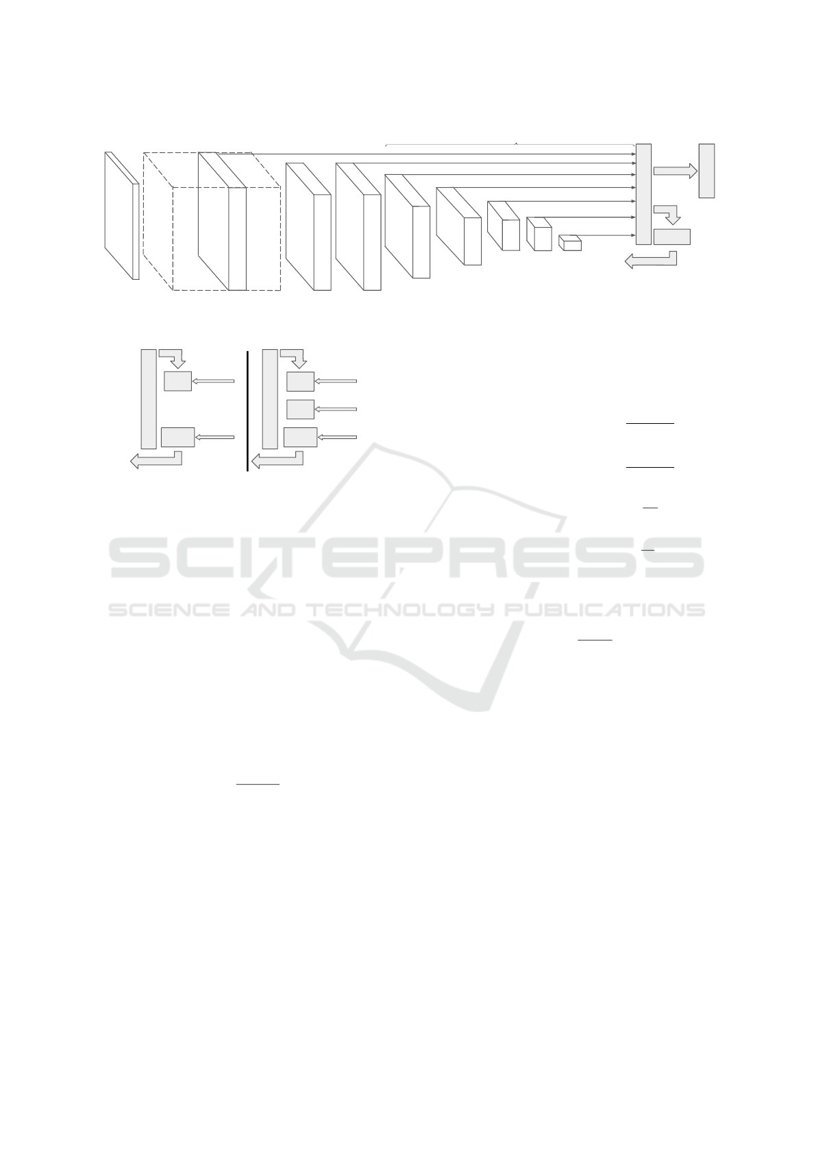
A. Modiﬁed SSD Detector. Similar to the SSD de-

tector, our SSD-ML detector consists of a CNN base

network and a detection head (see Figure 1). The

input of the detector is an image of 512 × 512 pix-

els. The VGG16 (Simonyan and Zisserman, 2014)

base network computes image features. Detection

boxes are predicted by detection heads that are cou-

pled to several layers from the base network and ad-

ditionally to down-scaled versions of the last feature

layer. Each detection head outputs possible detections

at ﬁxed positions in the image using so-called prior

boxes. The detection head estimates objectness o,

class conﬁdences [c

, c

, ..., c

] and location off-

sets δ(cx, cy, w, h) for each prior box in a feature layer.

These estimates are all predicted by a convolution

with a kernel of 3 × 3× the number of channels.

B. Prior Boxes. These boxes are associated to each

cell in a feature layer. The set of prior boxes Pr con-

tains boxes with varying aspect ratios and scales, to

cover all object sizes and shapes. The position of each

prior box relative to each cell is ﬁxed. Per feature

layer there are m × n locations (cells) and each loca-

tion has ||Pr|| prior boxes (the cardinality or size of

the set Pr). Detailed information of the individual as-

pect ratios and sizes of each prior box can be found in

the original SSD paper (Liu et al., 2016).

C. Matching. This step involves the matching be-

tween the set of prior boxes and ground-truth boxes,

which is carried out during training of the detector to

generate a set of positive matches Pos. Firstly, the

maximum overlapping prior box of each ground-truth

box is selected as a positive match. Next, all prior

boxes with a Jaccard overlap (IoU) of at least 0.5 with

a ground-truth box are also be added to the Pos set.

The set of positive matches is used for computing the

objectness, classiﬁcation and localization loss.

D. Negative Samples. These samples are collected

during training in a negative set Neg. This set consists

of all prior boxes that are not in the positive match-

ing set. This is a large set, since most of the prior

boxes will not match with any ground-truth box. To

compensate for the imbalance between the size of the

positive and negative sets, only the negatives with the

highest objectness loss (see below) are selected to be

used during training. The amount of negatives is cho-

sen to be a ratio of 3 : 1 with respect to the size of the

positive set.

E. Improvement of the Negative Set. In contrast with

the original SSD implementation, we propose to col-

lect negative samples per batch instead of per image.

The negative-to-positive ratio is kept the same, but

the negative samples may come from different im-

ages (within the same batch). This enables us to add

background images (without ground-truth bounding

boxes) containing complicated visual trafﬁc scenar-

ios. This improvement decreases the number of false-

positive detections when applying the detector at new

scenes containing never-before seen objects. For traf-

ﬁc detection, speciﬁc images containing empty high-

ways and empty city streets and crossings in all kinds

of weather conditions may be added to the training

set. Additionally, we propose to select negative sam-

ples more carefully by not selecting them in ignore

regions. Although these regions have to be manually

annotated in the training images, they are particularly

useful if only a part of the scene is annotated, or when

static (parked) vehicles are present in multiple train-

ing images. These regions should be ignored (see yel-

low regions in Figures 4 and 6) for negative mining.

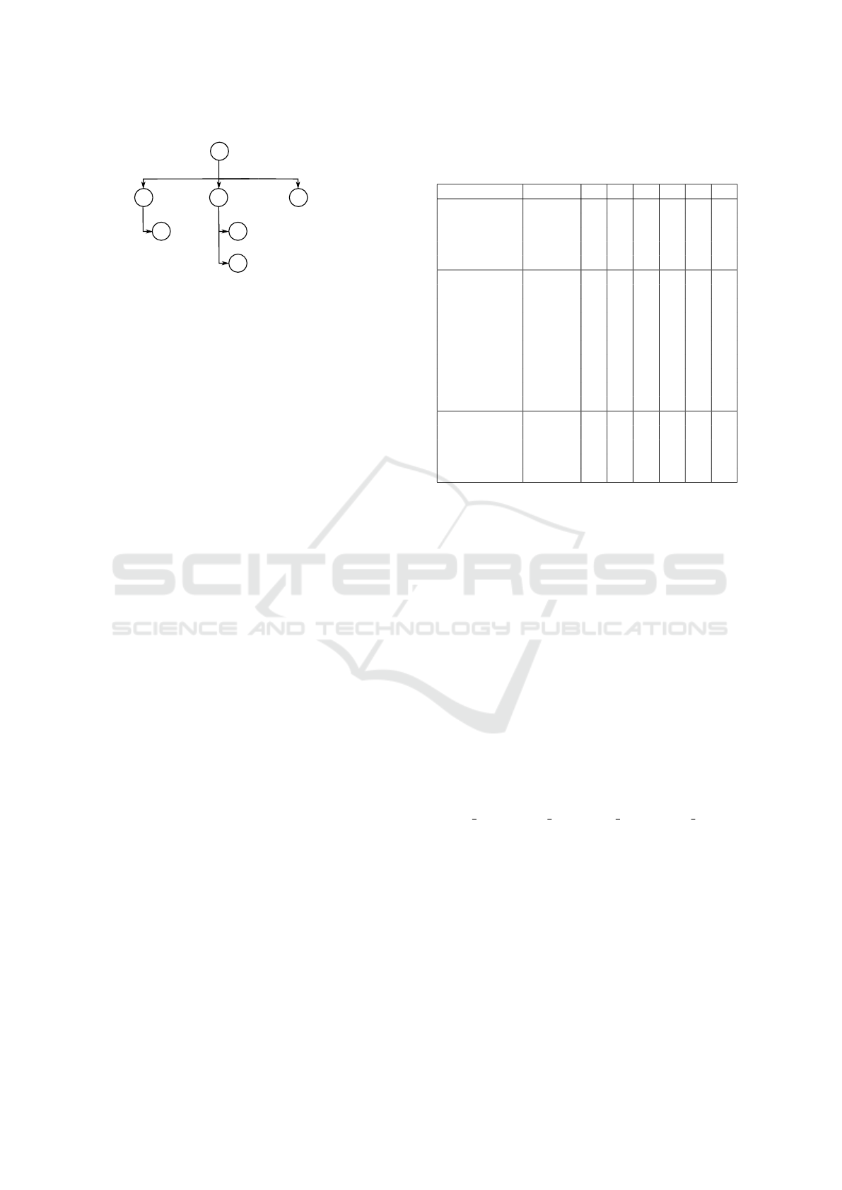
F. Objectness. The prediction of objectness is newly

introduced, compared to the original SSD implemen-

tation. The objectness loss L

ob j

and the classiﬁcation

loss L

class

replace and further detail the conﬁdence

loss L

con f

of the original SSD detector implementa-

tion (see Figure 2). The objectness estimate o

for

the i-th prior box is learned, using a binary logistic

loss function computed over the set of positive Pos

and negative Neg matches with ground-truth bound-

ing boxes. The objectness loss is then deﬁned by

ob j

(o) = −

∑

i∈Pos

log( ˆo

) −

∑

i∈Neg

log(1 − ˆo

), (1)

where ˆo

denotes the softmax function deﬁned by

ˆo

1 + e

−o

. (2)

G. Hierarchical Classiﬁcation. The classiﬁcation

conﬁdences are predicted per object category. Each

classiﬁcation category prediction score ˆc

, for the i-

th prior box for category p is determined by a binary

logistic loss. This means that each category predic-

tion output is independent from other category predic-

tions. The classiﬁcation loss L

class

is only computed

over the set of positive matches Pos between ground

truth and prior boxes. Let t

∈ {0, 1} be a binary in-

dicator for the i-th prior-box matching a ground-truth

box of category p or any of the subcategories of p and

VISAPP 2020 - 15th International Conference on Computer Vision Theory and Applications

252

VGG-16

through Conv5_3

Conv7

(FC7)

1024

Conv8_2

512

Conv9_2

256

Conv4_3

Conv10_2

256

512

Image

512

NMS

Conv11_2

Conv6

(FC6)

1024

Conv12_2

256

Conv 3x3x1024 Conv 1x1x1024

Conv 1x1x256

Conv 3x3x512-s2

Conv 1x1x128

Conv 3x3x256-s2

Conv 1x1x128

Conv 3x3x256-s2

Conv 1x1x128

Conv 3x3x256-s2

Conv 1x1x128

Conv 3x3x256-s2

Classiﬁer: Conv: 3x3x(4x(Classes + 4)

Classiﬁer: Conv: 3x3x(6x(Classes + 4))

Classiﬁer: Conv: 3x3x(5x(Classes + 4))

Classiﬁer: Conv: 3x3x(4x(Classes + 4))

Conv: 3x3x(2x(Classes + 4))

Detections: 8732

Extra Feature Layers

Deployment

Weights update

Loss

Training

Figure 1: The SSD detection model network design. Note that the loss function is visualized in more detail in Figure 2.

obj

loc

class

GT boxes

GT classes

Negatives

GT objects,

Weights update

Detections

loc

conf

GT boxes

Negatives

GT classes,

Weights update

Detections

SSD ML-SSD

Figure 2: Loss computation for SSD vs. ML-SSD model.

let Neg

⊂ Pos be a selection of ground-truth boxes

not of category p or any of its super-categories. This

notation is explained as follows. We wish to select

from the positive trafﬁc object set a speciﬁc set of ob-

jects that are a negative example of another class. The

samples in the negative set Neg

are selected based on

the dataset properties (see Table 1). The classiﬁcation

loss for category p is now deﬁned by

class, p

(t, c) = −

∑

i∈Pos

log( ˆc

))

−

∑

i∈Neg

log(1 − ˆc

(3)

where ˆc

is again the softmax function for this prior

box, giving

ˆc

1 + e

−c

. (4)

The total classiﬁcation loss becomes now the summa-

tion of all losses of the individual categories p.

H. Locations. The object locations are predicted

(similar to SSD) by estimating offsets δ(cx, cy, w, h)

for each prior box d in the set of prior boxes Pr at each

location in a feature layer. Parameters cx, cy, ... refer

to the offset in x dimension, y dimension, etc. Hence,

for a feature layer with dimensions m × n, there will

be ||Pr|| × m × n location estimates. The localization

loss is computed only over the set of positive matches

Pos between a predicted box l and a ground-truth box

g. More speciﬁcally, the offsets for the center (cx,

cy), width (w) and height (h) of the prior-box d are re-

gressed using a smoothing L1 loss function (Girshick,

2015), denoted by Smooth

(.), leading to:

loc

(l, g) =

∑

i∈Pos

(Smooth

−

− d

)

+Smooth

−

− d

)

+Smooth

− log

)

+Smooth

− log

)).

(5)

I. Training. The training of our model is carried

out by combining the different loss functions as a

weighted sum, resulting in

L(o, t, c, l, g) =

||Pos||

ob j

(o)

+β

∑

class, p

(t, c) + αL

loc

(l, g)).

(6)

If no object category is known in the ground-truth la-

bels, the classiﬁcation loss L

class

is set to zero. Con-

trary to the original SSD implementation where the

loss function is deﬁned to be zero when no objects are

present in an image during training, our loss function

is only deﬁned zero when no objects are present in a

complete batch due to our proposed negative mining

technique over a batch instead of per image.

J. Output. The output of the detection head is cre-

ated by combining the objectness conﬁdence, classi-

ﬁcation conﬁdences, location offsets and prior boxes

of all feature layers. These combinations are then

ﬁltered by a threshold on the objectness conﬁdence

followed by non-maximum suppression based on the

Jaccard overlap of the boxes. The output of the non-

maximum suppression results in the ﬁnal set of de-

tections. The conﬁdence per object category is deter-

mined by traversing down the class hierarchy, start-

ing with the objectness conﬁdence. The conﬁdence is

SSD-ML: Hierarchical Object Classiﬁcation for Trafﬁc Surveillance

253

Objectness

Van

Articulated-truck

Single-unit truck

Car

Truck

Bus

Figure 3: The proposed hierarchical categories for trafﬁc.

multiplied at each step with the parent category pre-

diction to ensure that a low parent category prediction

results in a low child category prediction.

4 TRAFFIC SURV. APPLICATION

Common datasets for evaluating object detection per-

formance focus on a wide range on object categories,

such as Pascal VOC (Everingham et al., 2012), Im-

ageNet (Russakovsky et al., 2015) and COCO (Lin

et al., 2014). These datasets contain a large amount of

images, with annotations of many object categories.

Although these datasets provide extensive benchmark

possibilities, they do not accurately represent trafﬁc

surveillance applications because of different view-

points and limited amounts of samples for speciﬁc

trafﬁc object classes. Datasets for trafﬁc surveillance

are typically created from ﬁxed surveillance cameras

also working in low-light conditions and under vary-

ing weather conditions, typically resulting in low-

resolution objects that are unsharp and often suffer

from motion blur. Recently, two large-scale traf-

ﬁc surveillance datasets have been published: UA-

DETRAC (Wen et al., 2015) and MIO-TCD (Luo

et al., 2018). Both datasets contain multiple vehicle

object categories and multiple camera viewpoints. In

this paper, we propose to combine these datasets for

training our object detector using our hierarchical ob-

ject category deﬁnition. The hierarchical categories

used in this paper are presented in Figure 3. We cre-

ate a new dataset for evaluation of the novel trained

object detector with hierarchical classiﬁcation.

4.1 Dataset 1: UA-DETRAC

The ﬁrst dataset used is the publicly available UA-

DETRAC (Wen et al., 2015), further referred to as

DETRAC in the remainder of this paper. This dataset

is recorded at 24 different locations in Beijing and

Tianjin in China at an image resolution of 960 × 540

pixels. Typical scenes contain multiple high-trafﬁc

lanes captured from a birds-eye view (see Figure 4).

Table 1: Mapping of the dataset labels to our hierarchical

categories. Samples are used as positive (P) or negative (N)

during training, otherwise they are ignored.

Label # 1 2 3 4 5 6

DETRAC

Car (5177) 479,270 P N N N

Van (610) 55,574 P N N P

Bus (106) 29,755 N N P

Other (43) 3,515 N P N

MIO

Artic. Truck 8,426 N P N N P

Bus 9,543 N N P

Car 209,703 P N N

Motorcycle 1,616

Mot. Vehicle 13,369

Non-Motor. 2,141

Pickup Truck 39,817 P N N

S. Unit Truck 5,148 N P N P N

Work Van 7,804 P N N P

Ours

Car 50,984 P N N

Bus 2,215 N N P

S. Unit Truck 1,422 N P N P N

Artic. Truck 2,420 N P N N P

The training set (abbreviated as trainset) contains 61

video clips with annotated bounding boxes. The

videos are sampled at a high temporal resolution

(25 fps), resulting in many images of the same physi-

cal vehicle. Each bounding box is classiﬁed into one

of four vehicle categories, i.e. car, bus, van, and other.

Table 1 describes the mapping of the DETRAC

dataset on our classiﬁcation tree. The numbers behind

the label names for DETRAC denote the number of

sampled physical objects. Note that in our hierarchy

‘Van’ is a sub category of ‘Car’ and in the DETRAC

set they are labeled individually, so that we can use the

DETRAC ‘Car’ label as negatives for our ‘Van’ cat-

egory. Visual inspection shows that the ‘Other’ cat-

egory in DETRAC contains various types of trucks.

Because the test set annotations have not been made

publicly available, we construct our own test set for

our experiments, based on a part of the original train-

ing set. The test set is created from the video clips

{MVI 20011, MVI 3961, MVI 40131, MVI 63525}

and consists of 4,617 images containing 54,593 an-

notations. The training set contains the remaining

77,468 images with 568,114 annotations.

4.2 Dataset 2: MIO-TCD

The MIO-TCD dataset (Luo et al., 2018), further re-

ferred to as MIO in the remainder of this paper, con-

sists of 137,743 images recorded by trafﬁc cameras all

over Canada and the United States. The images cover

a wide range of urban trafﬁc scenarios and typically

cover one or two trafﬁc lanes captured from the side

VISAPP 2020 - 15th International Conference on Computer Vision Theory and Applications

254

Figure 4: Example images from the UA-DETRAC dataset.

Figure 5: Example images from the MIO-TCD dataset.

of the road with a wide-angle lens, producing notice-

able lens distortion (see Figure 5). The image reso-

lution is generally low and varies from 342 × 228 to

720 × 480 pixels. Each vehicle annotation is catego-

rized into one of 11 vehicle categories, of which we

remove the ‘pedestrian’ and ‘bicycle’ categories, as

we focus on road trafﬁc. The remaining categories

are mapped to our hierarchical categories as shown

in Table 1. Note that the classes ‘Motorcycle’, ‘Mo-

torized Vehicle’ and ‘Non-Motorized Vehicle’ are not

assigned to any category, because they are used only

for the objectness prediction.

Similar to the DETRAC set, a small part of the an-

notations is used to create a test set. For this, we se-

lect every tenth image from the training set, resulting

in a validation set of 11,000 images containing 34,591

annotations. Our training set contains the remaining

99,000 images with 307,567 annotations.

4.3 Dataset 3: Our Constructed Dataset

Our dataset is considerably smaller in size than

the DETRAC and MIO datasets, but contains high-

resolution images of 1280×720 and 1920×1080 pix-

els, recorded from typical surveillance cameras mon-

itoring urban trafﬁc in Europe. The captured scenes

Table 2: Our testing set categories (note that class 1 and 2

include their sub-classes).

# Label Samples %

1 Car (incl. 4) 5681 89.3%

2 Truck (incl. 5, 6) 438 6.9%

3 Bus 244 3.8%

4 Van 590 9.3%

5 Single-unit truck 160 2.5%

6 Articulated truck 236 3,7%

Total objects 6363 100.0%

Figure 6: Example images from our dataset.

contain trafﬁc crossings, roundabouts and highways.

In total, 20,750 images are captured at 12 different

locations in various light and weather conditions. All

images are manually annotated with object bounding

boxes and labels.

The dataset is split into a test set of 2,075 ran-

domly selected images, containing 6,363 bounding

box annotations. Each bounding box is assigned one

of the hierarchical categories according to Table 1.

Note that the ‘Van’ category is not annotated in our

training set and that only the subcategories of ‘Truck’

are present. The training set contains 90,237 annota-

tions in 18,675 images. In our test set, we manually

annotated the ‘Van’ category to enable validating our

detector. Table 2 shows the test set distribution.

To validate the performance of our newly intro-

duced hard-negative mining method over background

images, a dataset containing only background is cre-

ated. This dataset is created by computing the pixel

median over every 100 images in every scene in our

dataset. This results in 154 background images of

scenes in our trainset. This background set is rela-

tively small compared to other datasets used for train-

ing, therefore each background image is sampled 10

times more often than other images during training.

SSD-ML: Hierarchical Object Classiﬁcation for Trafﬁc Surveillance

255

5 EXPERIMENTAL RESULTS

The trafﬁc detection and classiﬁcation performance of

the detector has been experimentally validated. The

detector is incrementally trained by iteratively adding

datasets, while evaluating performance over our ﬁxed

test set. We ﬁrst present the evaluation criteria and the

details of the training procedure. Object detection is

then evaluated, followed by an in-depth discussion of

hierarchical classiﬁcation results.

5.1 Evaluation Metrics

Evaluation of detection performance is carried out us-

ing the Average Precision (AP) metric as used in the

PASCAL VOC challenge (Everingham et al., 2012).

This metric summarizes a recall-precision curve by

the average interpolated precision value of the posi-

tive samples. Recall R(c) denotes the fraction of ob-

jects that are detected with a conﬁdence value of at

least c. An object is detected if the detected bound-

ing box has a minimum Jaccard index of 0.5 with the

ground-truth bounding box, otherwise a detection is

considered incorrect. Precision P(c) is deﬁned as the

fraction of detections that are correct with a conﬁ-

dence value of at least c. The average precision AP

is computed as the area Under the recall-precision

curve. To evaluate the combined performance of our

hierarchical classiﬁcation system, the mean Average

Precision (mAP) is used, calculated as the mean of

the average precision scores per object category.

5.2 Training Details

Our SSD-ML detector is trained using the following

training parameters. We apply 120,000 iterations on

batches of 32 images with a learning rate of 4 ×10

−4

while decreasing with a factor of 10 after 80k and

100k iterations using stochastic gradient descent. We

set α to unity and β to 0.5 (Eq. (6)).

5.3 Vehicle Detection: Effect of Datasets

In this ﬁrst experiment we perform measurements

with the baseline SSD detector for a single-class de-

tection problem on all datasets. This provides insight

in the variations of vehicles between the datasets, as

they are recorded in different countries with different

camera viewpoints. The original SSD implementation

cannot be trained with our hierarchical object cate-

gories. It is not possible to deﬁne a single (non hier-

archical) class deﬁnition that is valid for all datasets.

To evaluate the detection performance for all vehicle

types, we propose to evaluate the vehicle detection

Table 3: Average precision for object detection.

Trainset Model DETRAC MIO Ours

DETRAC SSD 90.6 48.4 77.8

SSD-ML 97.4 59.7 83.8

MIO SSD 87.4 87.8 78.4

SSD-ML 92.6 88.4 83.6

Ours SSD 89.8 42.9 90.5

SSD-ML 95.7 61.8 96.4

task, using the average precision of the single-class

objectness scores (vehicle vs. background).

The detection results on the DETRAC, MIO and

our dataset are presented in Table 3. Each row

presents a detector trained on ‘trainset’ and evalu-

ated over all datasets. Comparing the original SSD

implementation (SSD) with our proposed detection

model (SSD-ML) shows that our detector performs

signiﬁcantly better when trained on DETRAC or our

dataset. This is not expected, as the different loss

functions (softmax vs. logistic) have similar be-

haviour for a single-class problem. However, the DE-

TRAC dataset and our dataset contain annotated ig-

nore regions, which are regions containing vehicles

that are not annotated. Our implementation does not

allow hard-negative mining in these areas (see Sec-

tion 3), which results in the above-mentioned signiﬁ-

cant improvement.

The detector trained on DETRAC performs well

on our dataset (83.8%), while it has much lower per-

formance (48.4% and 59.7%, respectively) on the

MIO dataset. The detectors trained on MIO perform

well on all datasets. We expect this originates from

the large amount of camera viewpoints and vehicle

variations in the MIO dataset. Although the DE-

TRAC set is two times larger, it contains less vari-

ation, signiﬁcantly hampering detection performance

on MIO (59.7%).

When trained on our dataset, the detector obtains a

much higher AP on our test set (90.5% and 96.4%, re-

spectively). Although our dataset is smaller, it covers

the visual variation contained in the DETRAC set and

obtains comparable performance (95.7%). In compar-

ison to MIO, our dataset lacks variation in viewpoints,

resulting in a performance drop (61.8%). In addition,

we expect that the detector cannot robustly detect the

vehicles with limited image quality, large variations in

viewpoint, image roll and lens distortion in the MIO

set. This experiment shows that our dataset is sufﬁ-

ciently large to train a good vehicle detector (single-

class) when the camera viewpoints are similar (DE-

TRAC), but covers insufﬁcient viewpoint variations

for robust detection on MIO.

VISAPP 2020 - 15th International Conference on Computer Vision Theory and Applications

256

5.4 Vehicle Detection: Effect on Classes

In this experiment the performance of our detector is

evaluated in more detail. Using our single-class vehi-

cle detector, we now evaluate the performance for the

different vehicle classes and investigate the effect of

combining training datasets. We report the recall of

the different classes, measured at a ﬁxed threshold at

90% precision.

The obtained results are reported in Table 4. We

focus on the contribution of the additional training

sets on the detection performance on our dataset and

the effect on the different vehicle categories. Train-

ing with the DETRAC and MIO datasets individually

results in an AP of 83%, while their combination im-

proves the AP to 86.3%. The recall per object cat-

egory shows that the MIO dataset has high recall for

trucks and busses and lower recall for cars/vans, while

the DETRAC dataset has high recall for cars/vans and

lower for trucks and busses. Because our test set (Ta-

ble 2) is highly imbalanced, the car category domi-

nates the combined AP. This is as expected, as the

DETRAC dataset only contains a small amount of

trucks. Combining DETRAC and MIO leads to an

improved or similar performance on each of the dif-

ferent classes.

Adding our background set improves AP to

87.6%. Although the background set does not con-

tain any objects, it allows for better hard-negative har-

vesting, causing less false positive detections. This

can be observed speciﬁcally for the category ‘Single

Unit Truck’ (and ‘Truck’), which increases by 3.4%

(2.8%). Although it seems that the detection of this

class is better, this improvement originates from the

fact that the overall precision improves (less false de-

tections because of explicit background data). This

automatically results in a higher recall (at precision

90%) which has most effect for objects with a low

objectness score, single-unit trucks in this case.

The detector trained on only our dataset outper-

forms the other combinations with an AP of 96.4%, it

also outperforms the detector trained on the combina-

tion of DETRAC, MIO and our dataset. However, the

performance of this detector has low detection perfor-

mance on the MIO dataset (61.8% AP score). Our

training set is small which could lead to over-ﬁtting.

Overall, training with more data results in better de-

tection performance on all datasets.

5.5 Vehicle Classiﬁcation

The ﬁnal experiment concentrates on the classiﬁca-

tion performance. Using the models trained and pre-

sented in the previous experiments, the classiﬁcation

performance is measured per object class in our hier-

archical tree. The average precision is measured for

each object class individually on our testing set and

summarized by the mean Average Precision (mAP).

Table 5 presents the results. The classiﬁcation per-

formance when trained on the DETRAC set is rather

low for the ‘Truck’,‘Van’ and ‘Bus’ categories. Low

performance for truck classiﬁcation is expected, since

there are only few trucks (43) present in the DETRAC

dataset. Single-unit and articulated trucks are not la-

beled and thus not trained, but a prediction is always

made by the detection model for this class, so noise

in the network leads to classiﬁcations with very low

score. The ‘Bus’ category has an AP of 53.3% de-

spite the high amount of busses in the dataset. Visual

inspection shows that many false positive classiﬁca-

tions for busses originate from trucks in the testing

set, causing low precision. The low performance for

vans results from many larger vehicles, which are be-

ing falsely classiﬁed (such as station-wagons).

When training only with the MIO dataset, the AP

for trucks, busses and the sub-classes ‘Single-Unit

Truck’ and ‘Articulated truck’ are higher compared to

the DETRAC set, but the AP value remains still low.

Only for vans, the performance is lower, which is ex-

pected because no negative samples are available dur-

ing training (See Table 1) causing many false-positive

classiﬁcations. When combining DETRAC and MIO

for training, this results in a minor improvement com-

pared to DETRAC only and a small loss in perfor-

mance compared to MIO only, where the ‘Van’ class

is an exception and improves slightly from this com-

bination. Similar to the detection performance, when

background images are added to the training set, the

overall average precision increases.

Training with our dataset results in high average

precision for all object categories except ‘Van’. Vans

are not present in our training dataset (See Table 1).

The detector trained on all combined datasets

achieves highest mean average precision. Especially

for vans, it obtains a high average precision compared

to the rest of the trained detectors. This is remark-

able, because vans are not labeled in our training set.

Visual inspection of the false positives for the detec-

tor trained with DETRAC, MIO and our background

set, compared to the detector trained with all datasets,

shows that busses cause confusion with cars/vans in

our testing set. So by adding our training dataset

which contains relatively many busses, the car AP im-

proves, and thereby also the the classiﬁcation score

of vans and busses. The classiﬁcation performance

for the ‘Single-Unit Truck’ category is lower than

training only with our dataset, hinting that the other

datasets actually do not provide correct information

SSD-ML: Hierarchical Object Classiﬁcation for Trafﬁc Surveillance

257

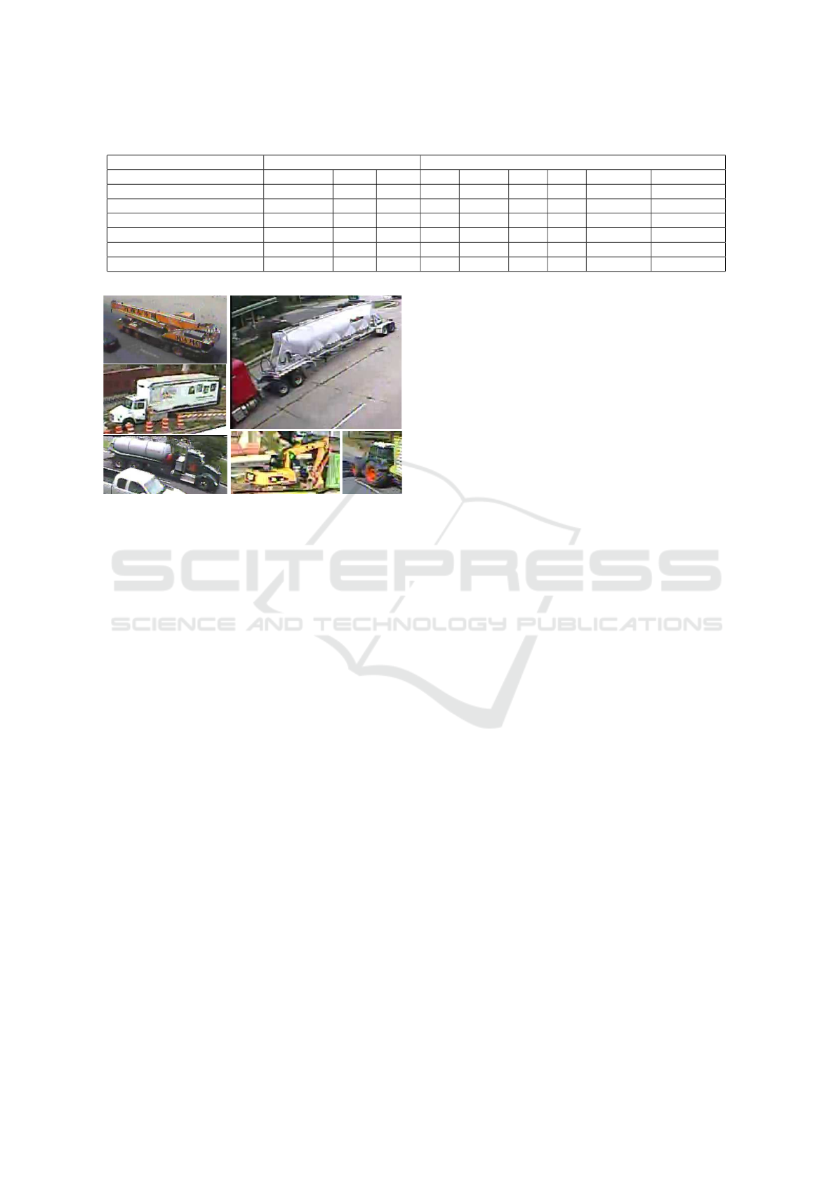
Table 4: Average precision evaluation of SSD-ML objectness score (detection only, ignoring classiﬁcation).

Trainset Average Precision Recall per category on Ours@P90

DETRAC MIO Ours Car Truck Bus Van A. Truck S.U. Truck

DETRAC 97.4 59.7 83.8 59.6 56.5 77.5 79.6 55.6 58.1

MIO 92.6 88.4 83.6 57.2 65.5 80.4 77.3 64.4 68.2

DETRAC + MIO 97.7 89.6 86.3 61.1 65.5 80.8 79.8 65.0 68.2

DETRAC + MIO + Backgr. 98.1 89.8 87.6 62.9 68.3 82.6 81.8 66.3 71.6

Ours 95.7 61.8 96.4 72.8 77.6 88.4 87.7 74.4 78.8

DETRAC + MIO + Ours 97.9 87.5 95.6 71.4 75.7 88.8 86.9 72.5 76.7

Figure 7: ‘Single-Unit Truck’ examples in MIO.

for single-unit trucks. The DETRAC set does not con-

tain samples of single-unit trucks. Visual inspection

of the class images for MIO shows a variation of large

vehicles that do not ﬁt the remaining class categories

of MIO, such as excavators and tractors (see Figure7).

6 DISCUSSION

In our experiments, we have observed that combin-

ing the datasets is not trivial. First, labeled object

categories in each dataset should be labeled consis-

tently. Samples for the ‘Single-Unit Truck’ category

in the MIO dataset are different vehicle types when

comparing the same labels in our dataset. More-

over, vehicle models are different in Europe, Asia and

USA/Canada. Trucks are larger in the USA compared

to Europe and Asia. For example, pick-up trucks in

America are considered cars, whereas in Europe they

are often considered trucks.

Because we have separated the vehicle presence

and classiﬁcation tasks, inconsistent sub-labels of a

class can still be used to improve object localization

and classiﬁcation of the (super-)class. For example, in

our case the category ‘Single-Unit Truck’ in the MIO

dataset can be used for training our objectness pre-

diction without any changes to the dataset to improve

detection performance of the general vehicle class.

The public datasets used in this paper did not

make their test set labels publicly available. We man-

ually extracted part of the training set for testing,

thereby introducing similar camera viewpoints in the

test sets. This poses a risk for over-ﬁtting our model.

This aspect of limited camera viewpoints may hold

for all datasets including our own, which is difﬁcult to

avoid for surveillance sets that are always constructed

from ﬁxed-camera videos with a ﬁxed background

and limited viewpoint variation. Gathering new im-

age material is difﬁcult and labor intensive, resulting

in a limited number of camera viewpoints. Separating

all images from a speciﬁc camera viewpoint in a test

set is therefore not desired, as it reduces the training

set signiﬁcantly.

7 CONCLUSIONS

In this paper, we have proposed a novel detection

system with hierarchical classiﬁcation, based on the

state-of-the-art Single-Shot multibox Detector (SSD).

Inspired by the recent You Only Look Once (YOLO)

detector, prediction of object presence is learned sep-

arately from object class prediction. Our implementa-

tion uses logistic binary instead of softmax classiﬁca-

tion. Independent training of the classiﬁcation classes

allows combining datasets that are not labeled with a

complete set of object classes. Additionally, we em-

ploy so-called ignore regions in the datasets during

training, which are regions containing unannotated

vehicles and describe areas where no negative sam-

ples are mined. Moreover, we use an improved hard-

negative mining procedure by selecting examples in a

training-batch instead of per image.

We have experimented with this novel SSD-ML

detector for trafﬁc surveillance applications and com-

bined different public surveillance datasets with non-

overlapping class deﬁnitions. The UA-DETRAC and

MIO-TCD datasets are combined, together with our

newly introduced dataset. In our ﬁrst experiment, the

effect of the dataset on the detector performance is

evaluated. Our new method for negative mining in

unannotated areas signiﬁcantly improves the detec-

tion compared to the original SSD detector. We show

VISAPP 2020 - 15th International Conference on Computer Vision Theory and Applications

258

Table 5: Mean Average Precision and Average precision per object category, tested on our dataset.

Trainset mAp Car Truck Bus Van S.U. Truck A. Truck

DETRAC 27.1 76.4 15.6 53.3 14.9 1.1 1.5

MIO 47.4 78.3 60.7 70.1 4.0 16.4 54.9

DETRAC + MIO 46.1 81.9 51.1 68.5 26.6 12.0 36.3

DETRAC + MIO + Background 49.7 82.5 62.6 69.6 19.4 13.5 50.4

Ours 77.2 95.5 97.7 85.6 2.9 84.8 96.7

DETRAC + MIO + Ours 78.6 94.5 93.4 84.4 62.2 48.3 88.7

that our dataset and the larger UA-DETRAC dataset

result in similar detection performance, implying that

both sets contain sufﬁcient information to train a de-

tector with similar high performance for localization.

In a second experiment, we have investigated the

effect of incrementally adding more datasets and have

shown that the best performance is obtained when

combining all datasets for training. Although the

MIO-TCD dataset has very different viewpoints, im-

age quality and lens distortion, it offers a large varia-

tion in the data with a high number of labels, so that it

still contributes visually to the detection of the other

viewpoints. The ﬁnal system obtains a detection per-

formance of 96.4% average precision, improving with

5.9% over the original SSD implementation mainly

caused by our hard-negative mining.

Finally, we have measured the classiﬁcation per-

formance of our hierarchical system. The effect of

incrementally adding more datasets reveals that the

best performance is obtained when training with all

datasets combined. By adding hierarchical classiﬁca-

tion, the average classiﬁcation performance increases

with 1.4% to 78.6% mAP. This positive result is based

on combining all datasets, although label inconsisten-

cies occur in the additional training data. Note that the

overall detection performance drops 0.8% in this case.

Since vans are not labeled as such in our dataset, we

have additionally trained our classiﬁer for vans with

labels from the UA-DETRAC and MIO-TCD dataset.

The resulting detector obtained a decent classiﬁcation

performance of 62.2% for vans, on our separate test

set. We have shown that non-labeled object classes

in actually existing datasets can be learned using ex-

ternal datasets providing the labels for at least those

classes, while simultaneously also improving the lo-

calization performance.

REFERENCES

Everingham, M., Van Gool, L., Williams, C. K. I., Winn,

J., and Zisserman, A. (2012). The PASCAL Visual

Object Classes Challenge 2012 (VOC2012) Results.

Fan, Q., Brown, L., and Smith, J. (2016). A closer look

at faster r-cnn for vehicle detection. In 2016 IEEE

Intelligent Vehicles Symposium (IV), pages 124–129.

Girshick, R. (2015). Fast R-CNN. In ICCV.

Girshick, R., Donahue, J., Darrell, T., and Malik, J. (2014).

Rich feature hierarchies for accurate object detection

and semantic segmentation. In IEEE CVPR.

He, K., Gkioxari, G., Doll

ar, P., and Girshick, R. (2017).

Mask R-CNN. In ICCV.

Lin, T.-Y. et al. (2014). Microsoft COCO: Common objects

in context. In ECCV, pages 740–755. Springer.

Liu, W., Anguelov, D., Erhan, D., Szegedy, C., Reed, S.,

Fu, C.-Y., and Berg, A. C. (2016). Ssd: Single shot

multibox detector. In ECCV, pages 21–37. Springer.

Luo, Z. et al. (2018). MIO-TCD: A new benchmark dataset

for vehicle classiﬁcation and localization. IEEE Trans.

Image Processing, 27(10):5129–5141.

Lyu., S. et al. (2018). UA-DETRAC 2018: Report

of AVSS2018 IWT4S challenge on advanced trafﬁc

monitoring. In 2018 15th IEEE International Con-

ference on Advanced Video and Signal Based Surveil-

lance (AVSS), pages 1–6.

Redmon, J., Divvala, S., Girshick, R., and Farhadi, A.

(2016). You only look once: Uniﬁed, real-time ob-

ject detection. In CVPR, pages 779–788.

Redmon, J. and Farhadi, A. (2017). Yolo9000: Better,

faster, stronger. In CVPR, pages 6517–6525.

Ren, S., He, K., Girshick, R., and Sun, J. (2015). Faster R-

CNN: Towards real-time object detection with region

proposal networks. In NIPS.

Russakovsky, O. et al. (2015). ImageNet Large Scale Vi-

sual Recognition Challenge. International Journal of

Computer Vision (IJCV), 115(3):211–252.

Simonyan, K. and Zisserman, A. (2014). Very deep con-

volutional networks for large-scale image recognition.

arXiv preprint arXiv:1409.1556.

Sivaraman, S. and Trivedi, M. M. (2013). Looking at vehi-

cles on the road: A survey of vision-based vehicle de-

tection, tracking, and behavior analysis. IEEE Trans.

Intelligent Transportation Systems, 14(4):1773–1795.

Tian, Z., Shen, C., Chen, H., and He, T. (2019). FCOS:

Fully convolutional one-stage object detection. In

ICCV.

Wen, L., Du, D., Cai, Z., Lei, Z., Chang, M., Qi, H., Lim,

J., Yang, M., and Lyu, S. (2015). UA-DETRAC: A

new benchmark and protocol for multi-object detec-

tion and tracking. arXiv CoRR, abs/1511.04136.

SSD-ML: Hierarchical Object Classiﬁcation for Trafﬁc Surveillance

259