
Superpoints in RANSAC Planes: A New Approach for Ground Surface
Extraction Exemplified on Point Classification and Context-aware
Reconstruction
Dimitri Bulatov
1 a
, Dominik St
¨
utz
1
, Lukas Lucks
1
and Martin Weinmann
2
1
Fraunhofer Institute for Optronics, System Technologies and Image Exploitation (IOSB),
Gutleuthausstrasse 1, 76275 Ettlingen, Germany
2
Institute of Photogrammetry and Remote Sensing, Karlsruhe Institute of Technology (KIT),
Englerstr. 7, 76131 Karlsruhe, Germany
Keywords:
Point Cloud, Classification, Surface Reconstruction, Superpoints.
Abstract:
In point clouds obtained from airborne data, the ground points have traditionally been identified as local
minima of the altitude. Subsequently, the 2.5D digital terrain models have been computed by approximation
of a smooth surfaces from the ground points. But how can we handle purely 3D surfaces of cultural heritage
monuments covered by vegetation or Alpine overhangs, where trees are not necessarily growing in bottom-to-
top direction? We suggest a new approach based on a combination of superpoints and RANSAC implemented
as a filtering procedure, which allows efficient handling of large, challenging point clouds without necessity
of training data. If training data is available, covariance-based features, point histogram features, and dataset-
dependent features as well as combinations thereof are applied to classify points. Results achieved with
a Random Forest classifier and non-local optimization using Markov Random Fields are analyzed for two
challenging datasets: an airborne laser scan and a photogrammetrically reconstructed point cloud. As an
application, surface reconstruction from the thus cleaned point sets is demonstrated.
1 INTRODUCTION
Dense 3D point clouds are more easily accessible than
ever before thanks to increasingly cheap laser tech-
nologies and to advanced pipelines for photogram-
metric reconstruction, available for commercial and
non-commercial use. It is thus not surprising they
find many applications in construction industry, civil
engineering, and, as a particular focus of this work,
in cultural heritage preservation. Here the application
fields range from documentation to monitoring and
from uncovering testimonies of the historic civiliza-
tion (Evans et al., 2013) to elaboration of solutions
for preservation of monuments of cultural heritage as
was the case for the HERACLES project funded by
the Horizon 2020 research and innovation program of
the European Union. To perform analysis of erosions
within in-situ measurements, a large-scale prepara-
tion of data and identification of particularly threat-
ened spots is required (Bulatov et al., 2018).
All these applications underline a growing need
for innovative methods for the treatment and analy-
sis of large 3D point clouds. In particular, for moni-
a
https://orcid.org/0000-0002-0560-2591
toring of cultural heritage, it is important to identify
vegetation areas to be able to differentiate between
those points changing seasonally and those indicat-
ing deterioration of substance. Trees and bushes, not
much relevant for model representation and monu-
ment preservation, should ideally be omitted or mod-
eled by generic models (Lafarge and Mallet, 2012),
while those parts of the scene which are covered by
vegetation may be closed using methods of geometric
inpainting (Guo et al., 2018). This is done because,
on the one hand, data exchange between multinational
partners working on the aforementioned project (Bu-
latov et al., 2018) has turned out to be a non-negligible
issue, and, on the other hand, a gap-free surface for
building models has to be obtained.
The necessary requisite of this semantic surface
modeling representation of a point cloud, namely its
classification into semantic categories (terrain, vege-
tation, building parts), must be addressed. Still, in
the literature, see Section 2, we gained an impres-
sion that many previous works relied on a sampling
of the point cloud into an elevation map, that is, as-
signing a z-value to a pair (x,y) within a discrete rect-
angular grid. This is a limitation in presence of ver-
tical walls, balconies, or other purely 3D structures
Bulatov, D., Stütz, D., Lucks, L. and Weinmann, M.
Superpoints in RANSAC Planes: A New Approach for Ground Surface Extraction Exemplified on Point Classification and Context-aware Reconstruction.
DOI: 10.5220/0008895600250037
In Proceedings of the 15th International Joint Conference on Computer Vision, Imaging and Computer Graphics Theory and Applications (VISIGRAPP 2020) - Volume 1: GRAPP, pages
25-37
ISBN: 978-989-758-402-2; ISSN: 2184-4321
Copyright
c
2022 by SCITEPRESS – Science and Technology Publications, Lda. All rights reserved
25

where no such function z(x,y) exists. Another limita-
tion is the necessity to differentiate between different
sources of data (LiDAR-based or stemming from a
photogrammetric reconstruction, among others). This
brings about, finally, the shortcomings of the point
cloud itself: variable, sometimes very low point den-
sity, noise, and outliers. In order to cope with this,
a particular data structure, called superpoints, will
be proposed in Section 3. This structure, robust to
the variable point density, will allow to decrease the
data volume considerably. Using RANSAC, we will
find out which superpoints lie in a dominant plane,
which will allow for a large-scale separation of ter-
rain and non-terrain points without the necessity of
training data generation. Thus, the approach called
SIRP (superpoints in RANSAC plane) is the main
contribution of this article because of being success-
ful, in particular, for challenging scenarios of explicit
three-dimensional structure of the data: The abso-
lute orientation of the planes, or vertical axis direc-
tion, is not supposed, and thus, invariance of SIRP
related to rotations is guaranteed. The superpoints
in planes are clustered and the corresponding points
may be (re)labeled interactively and clusterwise, in
order to correct gross errors or to generate training
data for more than two classes, if necessary. Given
the availability of training data, supervised classifi-
cation approaches may be applied. For a fair com-
parison of their performance with SIRP and as an-
other, minor contribution of this article, we will con-
centrate on two important sets of rotational invariant
features: covariance-based features and those based
on point feature histograms. Additionally to these
features, we will marginally refer to those tailored to
the datasets or applications (source- and application-
dependent). The third important contribution is pre-
sented with post-processing using non-local optimiza-
tion on Markov Random Fields. In Section 4, the per-
formance of SIRP, source-independent features and
post-processing using non-local optimization will be
evaluated. Filtering out non-terrain points allows for
a context-aware surface reconstruction using Poisson
method, which will be presented as an example of an
application. Finally, in Section 5, we will summarize
our work and outline future research directions.
2 RELATED WORK
There is a large amount of methods on 3D point clas-
sification. Roughly, it was the tendency until 2005
to use rule-based approaches for separation, in par-
ticular, of terrain points from the off-terrain regions.
The pioneering work (Kraus and Pfeifer, 1998) for ex-
tracting ground surface in predominantly flat terrain
presupposes an iterative procedure for robust plane
fitting under the constraint that the off-terrain points
may lie far above but not far below the plane. Since
then, other contributions based on slope-based filter-
ing (Vosselman, 2000), progressive morphological fil-
tering (Zhang et al., 2003) and hierarchical filtering
(Mongus and
ˇ
Zalik, 2012), as well as contour analysis
(Elmqvist et al., 2001), have been developed to obtain
the ground surface in non-flat terrain as well. This
last method, briefly summarized as a two-step proce-
dure consisting of ground point detection and surface
fitting, can be considered as a state-of-the-art identi-
fication of ground in 2.5D data because, since then,
related works are striving to optimize the two steps to
make them less sensitive to outliers, sudden elevation
changes, etc. (Mousa et al., 2019; Perko et al., 2015).
However, both steps of this context will fail for pure
3D point clouds.
With more classes to be differentiated and with
the increasingly challenging scenarios, also the num-
ber of criteria, or features, for differentiation must in-
crease and the manually set thresholds have gradually
been replaced by those computed automatically from
the previously selected training data. In pure 3D point
clouds, using the features planarity, elevation, scat-
tering, and linear grouping has been proposed (La-
farge and Mallet, 2012), and one major concern here
is about the choice of the activation parameters σ for
each of these features. In (West et al., 2004), the
features based on the eigenvalues of the covariance
matrix (also called structure tensor) over the point’s
neighbors are introduced. The thus obtained features
are scale-, translation- and rotation-invariant. They
are used in (Gross and Thoennessen, 2006; Lalonde
et al., 2005; Weinmann, 2016) and other investiga-
tions in order to classify points from remote sensing
data with respect to their geometric saliency. With an
interest in theoretical bounds for neighborhood size
and shape, the results of experimentation with dif-
ferent neighborhood types are presented in (Wein-
mann, 2016; Weinmann et al., 2017): the involved
neighborhood types are given by the k nearest neigh-
bors (kNN), spherical neighborhoods and cylindrical
neighborhoods with varying values of k and varying
radii, while the cylinder height is set to infinity. From
the eigenvector corresponding to the smallest eigen-
value, the information about the local normal vector
can be derived and, similarly, the distribution of the
normals within the neighborhood can be explored. In
(Rusu et al., 2009), angular differences between lo-
cal coordinate systems of pairs of neighboring points
are computed. For each pair of points, there are three
angles, and for a fixed point with k neighbors, these
GRAPP 2020 - 15th International Conference on Computer Graphics Theory and Applications
26

differences are normalized according to the number
of neighbors and collected into three histograms. An
injective mapping from three integer numbers (bins)
into the one-dimensional index constitutes the com-
putation of Point Feature Histograms (PFHs). This
histogram has one peak in case of an approximately
planar surface point and a uniform distribution for
volumetric point clouds typical for trees.
As one can see from the survey in (Hana et al.,
2018), PFHs are not the only descriptors for point
clouds. This concept gives a hint that successive as-
sessing attributes of neighbors is a key to successful
machine understanding of data, even in challenging
scenarios, since it allows to capture context informa-
tion over considerable shapes. In 2D, this idea cul-
minated in approaches based on Convolutional Neu-
ral Networks. Nowadays, they are commonly applied
in 3D, among others, for classification tasks. Cur-
rently, PointNet++ is the state-of-the-art tool for point
classification and (Winiwarter et al., 2019) is the ex-
ample of application to remote sensing data. Here,
the visually impressive and quantitatively excellent
results are overshadowed by rather complex models
with many degrees of freedom, which in turn, require
an extensive training procedure, which may take long
for large-scale airborne laser scans.
One common observation of many recent works
is that the high number of 3D points and the point
density are not necessarily beneficial. The vast ma-
jority of points can be actually classified by rather
simple methods (thresholding) and hence, computa-
tion of higher-level features negatively affects the per-
formance efficiency. In (Rusu et al., 2008), it is
shown how to determine “interesting” points, CNN-
based methods like (Qi et al., 2017) perform pool-
ing, while the subsampling of a given point cloud into
voxels is proposed in (Hackel et al., 2016). From a
scale pyramid created by repeatedly down-sampling
the point cloud, a small number of nearest neighbors
is used at each scale for feature computation. The dif-
ference of this inspiring approach to ours is that we
neither compute a kd-structure for setting the voxels
nor use a rigid grid (as e.g. done in (Von Hansen,
2006) for point cloud registration purposes), but em-
ploy a flexible structure of superpoints in which points
are clustered using a fixed tolerance value. For the
particular task of separation of vegetation from the
ground, whereby the ground is not supposed to rep-
resent a horizontal surface but can be vertical or ex-
plicitly three-dimensional, we present the SIRP pro-
cedure specially tailored to this task. Basically, it is a
valuable tool for extraction of training data serving as
the basis of a successive supervised classification al-
gorithm, which is applied to the original point cloud.
3 METHODOLOGY
We start this section by describing two main ingre-
dients of the SIRP method, namely, superpoints and
dominant planes computed per superpoint. With these
information, we can easily take a decision for an in-
put point whether it belongs to the ground surface
or not (Section 3.3). Successively, we focus on fea-
ture extraction and describe the details of the super-
vised classification, including non-local optimization
on Markov Random Fields. An overview about im-
plementation details concludes this section.
3.1 Superpoints
For acceleration of upcoming computations and re-
duction of data, we introduce the concept of flexible
voxels or (3D) superpoints. The terminology may be
slightly misleading because, in the literature, and also
e.g. in the Point Cloud Library
1
, grouping takes place
using additional point features, such as Euclidean dis-
tance in normalized RGB space, while in our ap-
proach, feature computation takes place afterwards.
However, because of the functionality and because
such simpler features can be used at a later stage, we
will refer to superpoints from here on. This data struc-
ture allows identification of clusters of points within a
pre-defined tolerance ε and is, as we can see in Fig. 1,
left, more efficient as a voxel structure because there
are normally more voxels containing points than su-
perpoints. A fast computation of the structure may
by achieved by the following strategy: It starts by
converting the points scaled by the inverse value of
ε into integers and an injective mapping to a single
non-negative integer keeping in memory the indices:
{x,y,z} → { ˆx, ˆy, ˆz} → j = R
z
(R
y
ˆx + ˆy) + ˆz, (1)
where { ˆx, ˆy, ˆz} ∈ Z
3
+/0
:
ˆz = round(z/ε), ˆz = ˆz −min(ˆz),R
z
= max(ˆz)−min(ˆz),
and y and x are treated analogously. Then, sorting the
list and considering the differences of successive list
elements yields the break-points, between which the
list members of points belonging to the same super-
points are stored. Via the original indices, we finally
access the coordinates, from which we compute the
superpoints’ coordinates as centroids of voxels. In
the next step, we will compute the RANSAC plane
for the data points within a predefined radius around
the centroid. The radius should be a multiple of the
voxel size ε, so that the signatures of vegetation be-
come clear. This is visualized in Fig. 1, middle.
1
http://pointclouds.org/documentation/tutorials/
supervoxel clustering.php
Superpoints in RANSAC Planes: A New Approach for Ground Surface Extraction Exemplified on Point Classification and Context-aware
Reconstruction
27

Figure 1: Overview of the procedure for ground surface ex-
traction. In the left image, we compare the traditional voxel
structure (Von Hansen, 2006) with our superpoints (cyan
circles). Middle: Computation of RANSAC planes for each
superpoint and clustering procedure, whereby outliers are
indicated by yellow circles. Right: back-projection to the
original point cloud (red color for inliers).
3.2 RANSAC-based Plane Computation
Random Sample Consensus (Fischler and Bolles,
1981) is a well-known method for model fitting in
data with many outliers. Even though many modi-
fications of this method exist (Raguram et al., 2008),
we give a short description of our acceleration of this
method for the special case of plane fitting in the sense
that it only contains matrix multiplications. Thus, it
can be efficiently run with software optimized for ma-
trix processing (e.g. MATLAB), parallelized or even
implemented on GPUs.
The input 3D point cloud has a homogeneous
representation X =
{
(x
m
,y
m
,z
m
,1)
}
M
m=1
. Since three
points are required for a minimum sample for plane
computation, we consider U triplets of integer num-
bers T =
{
(a
u
,b
u
,c
u
)
}
U
u=1
, where all a
u
, b
u
, and c
u
lie between 1 and M. Other sampling strategies, such
as random choice of the first point followed by a
choice according to normal distribution for the two
remaining points, are possible, too. We define by
X
{i}
(T ),i = {1, ...,4} a U-tupil of 3 × 3 matrices. Its
columns correspond to the triplets of indexes in T and
their rows to X in which the i-th row has been omitted.
The computation of 4 ×U determinants (e.g., i = 4)
det
X
{4}
= x
a
y
b
z
c
− x
a
y
c
z
b
+ ... − x
c
y
b
z
a
(2)
is carried out simultaneously by element-wise multi-
plications and yields U plane hypotheses equations
p
i
= (−1)
i
det
X
{i}
, (3)
which are stored in a U ×4 matrix Π with Π
u,i
= p
i
(u)
from (3) and normalized normal vector. In order to
have a fixed number of hypotheses, U must be chosen
higher than this number. The degenerated configura-
tions can be filtered out easily since they yield p
i
= 0
for i = 1,...,4. In certain situations, additional filter-
ing is performed with respect to the slope of the plane
|p
3
| to discard nearly vertical surfaces. The U × M
matrix R
t
contains the residuals R thresholded by the
tolerance t:
R = Π · X → R
t
= R < t. (4)
This yields the number of inliers (column-wise sum
of R
t
) for all planes, and, therefore, the plane with the
highest number of inliers. Thus, RANSAC is now im-
plemented as a filtering procedure and multiplication
of two matrices. The output of this step is the infor-
mation whether the superpoint lies in its own plane or,
in other words, is part of the terrain. The remaining
superpoints are removed.
3.3 Cluster Analysis and
Back-propagation to the Point
Cloud
The goal of the previous step was to remove the mid-
dle and lower vegetation layers. The problem are the
tree canopies which may often be approximated by
planes. By considering clusters over remaining super-
points and suppressing clusters with less than 1000
members, we get rid of these superpoints as well.
Here, the number 1000 corresponds to the size of the
largest non-terrain objects divided by the voxel size ε.
Finally, the input point cloud is analyzed by con-
sidering the plane p = [v − n
T
v] through the super-
point v. The normal vector n
v
of p is obtained from
the covariance matrix (Weinmann, 2016) of a small,
fixed number of points in the cloud which are neigh-
bors of v, whereby the trade-off should be made be-
tween a better localization of the points and indepen-
dence on the local density of points. The third eigen-
value λ
3
is the measure of the local dispersion of this
plane. From a data point x, we search for the nearest
superpoints within a spherical neighborhood around
v and denote their number by N, whereby N ≤ 8 to
provide the analogy with image pixels. Each of these
superpoints has its own plane p
v
and we record the
number J of planes p of which x is an inlier (see Fig. 1
right). A point x is classified as terrain if and only if
J := # (d(x, p
v
) < t) > λ
3
· N. (5)
The best way to interpret this equation is to reflect a
borderline scenario. Is p the plane computed from an
absolutely planar point subset, then λ
3
= 0. In this
case, it is sufficient for a point x in the superpoint
merely to be the inlier of its own plane (p) because
the left hand side of (5) will be at least 1.
Using (5), we separate the terrain from non-terrain
objects (in particular vegetation) without the need for
training data. However, in case of multi-class prob-
lems, we need to specify training data labels, a feature
set, and a classifier. Since the availability of training
data depends on the dataset, we postpone this aspect
GRAPP 2020 - 15th International Conference on Computer Graphics Theory and Applications
28

until the results section and focus on the features and
learning algorithm in the remainder of this section.
3.4 Feature Extraction
There are two groups of generic features considered
in this work. On the one hand, the eight covariance-
based features are derived from the structure tensor,
already mentioned in Section 2: planarity, omnivari-
ance, linearity, scattering, anisotropy, eigenentropy,
curvature change, and sum of the eigenvalues (see
(Weinmann, 2016) for more details). These features
may be computed for different radii of the spheri-
cal/cylindrical neighborhood or number of neighbors
resulting from the kNN algorithm. On the other hand,
the Fast Point Feature Histograms (FPFHs) (Rusu
et al., 2009) yield 33 (alternative or additional) fea-
tures. They are known to be widely invariant to
changes of search radii and can be computed in lin-
ear time with respect to both the number of points in
the list and the neighborhood size. This is the big
difference to the originally implemented PFHs (Rusu
et al., 2008), where the dependence on the neighbor-
hood size is quadratic. Besides, we used multicore
processing in order to further accelerate the compu-
tations. Moreover, the points must be normalized to
have their centroid in the origin of the coordinate sys-
tem. It remains to note that the cardinality of point
neighbors required for computation of (F)PFHs must
not be smaller than that required for normal vector
computation. The dependence of the results and run-
time on different configurations of features will be
subject of evaluation.
Classification can be greatly improved if the prop-
erties of the underlying data are taken into account.
With available pulse number, intensities, and their dis-
tributions over neighborhoods in laser point clouds
as well as color values of points for results of pho-
togrammetric reconstruction, very valuable informa-
tion is given. In case of available color values, we nor-
malize them to have the unity L
1
-norm ([R,G, B] →
[R,G, B]/(R + G + B)), which allows for a better per-
formance in shadow regions (Weinmann and Wein-
mann, 2018). Besides, signed vertical distances of a
point to the 2.5D DTM surface computed by a state-
of-the-art method (Bulatov et al., 2012) provide large
values for overhanging points and medium values for
vegetation points.
3.5 Learning and Post-processing
Some of the features considered so far may be redun-
dant or even irrelevant for a particular classification
task. Ideally, the applied classifier should ignore these
features internally and show robust performance, even
if there is a moderate proportion of such bad features.
We use the Random Forest classifier (Breiman, 2001)
allowing the estimation of out-of-bag features. An ad-
ditional advantage of this classifier is that it is proba-
bilistic. This means that it outputs the probability of
a 3D point x to belong to a class l(x). This probabil-
ity P(l) corresponds to the percentage of trees in the
Random Forest voting for either class.
In the literature, it is popular to introduce a
smoothness prior that neighboring instances should
be encouraged to have the same labels. By interpret-
ing the instances as random variables on a Markov
Random Field (MRF), an energy function
E =
∑
x
−log P (l(x)) + λ
∑
y∈N (x)
(l(x ) 6= l(y))
(6)
is efficiently minimized using e.g. graph cuts (Boykov
et al., 2001), whereby we chose the alpha-expansion
algorithm available online (Delong et al., 2012). Note
that because of the two-class problem and a trivial
smoothness function, the result of the non-local op-
timization is the global minimum. The influence of
the smoothness parameter λ and the neighborhood N
will be addressed in the results section.
3.6 Implementation Details
In this section, we will refer to the choice of parame-
ter values. Some of them were mentioned in Sections
3.1-3.5 and remained fixed for both datasets of the re-
sults section. The voxel density ε depends on the size
of the smallest object to be detected and on the ex-
tension of the terrain that constitutes approximately a
plane. If ε is too small, then the terrain points will
be very scarce and if it is too large, then low vegeta-
tion, in particular, pasture may be excessively added.
Still, the choice of this parameter may deviate up to
20% with respect to the default value. We worked
with ε = 1 m and ε = 0.2 m for both point clouds –
the LiDAR-based respectively photogrammetric one
– which will be presented next. Surprisingly, not even
the computing time is dramatically dependent on this
parameter: With a larger ε, less superpoints must be
evaluated, on the one hand. On the other hand, they
contain more points, and since the value of U (number
of triplets in Section 3.2) corresponds to the number
of points, more time is needed. The RANSAC thresh-
old t was computed analytically depending on the su-
perpoint size and origin of the point cloud. It cor-
responds roughly to ε/2 while the radius for search
of points for RANSAC was 8ε. The clustering dis-
tance factor depends on the similarity of classes; val-
ues around 2ε are a good choice in our datasets, while
Superpoints in RANSAC Planes: A New Approach for Ground Surface Extraction Exemplified on Point Classification and Context-aware
Reconstruction
29

the cluster cardinality is supposed to rule out outliers.
Its value represents the trade-off between the size of
possible off-terrain objects (density of tree crowns)
and sudden changes of steepness of the terrain. As
a rule of thumb, if classes are badly separated, like
for photogrammetric point clouds because of over-
smoothing, one should tend to lower values of clus-
ter distances in order to prevent points from different
classes to lie in the same cluster. For well-separable
points, one could set the threshold for cluster distance
high. To compute the final plane, we used points in
the range of 2ε in the default case of nearest neighbors
in singular cases (isolated cluster center); the plane-
damping factor depends on the noise level. It should
be set to a higher value if parts of the terrain are less
likely to be approximated by a plane (stones on the
ground), or if less accurate points were produced by
the photogrammetric reconstruction. The number of
decision trees in Random Forests was set to 20 in all
experiments to guarantee relatively fast computation
with equal initial conditions for all experiments.
4 RESULTS
4.1 Datasets
The first discussed dataset is a point cloud obtained by
an airborne laser scan from an Alpine area in Southern
Germany. The main application here was the creation
of a photo-realistic database, which is usable for train-
ing and education in areas of disaster management
and other quick response applications (H
¨
aufel et al.,
2017). An interesting detail of this dataset, denoted
here and further as Oberjettenberg (as a neighboring
settlement is called), is that a 3D overhang does not
allow to describe the elevation z as a function of x and
y. Even though, according to the data provider, the
point density was 5 to 15 points per m
2
(while there
were some 81 millions of points in total), it varied
strongly from 10 to 100 responses; and, as Fig. 2, top,
shows, the regions belonging to the chinks and gorges
of the overhang are sparsely covered. To provide sur-
face reconstruction from an unorganized point cloud
(see e.g. (Guo et al., 2018) and references therein), it
is important to clean it from the points belonging to
trees. Around the overhang, deviations of growth di-
rections of trees from the vertical direction are almost
arbitrary, contrary to what we are used to in urban
scenery.
Our second dataset focuses on the medieval wall
surrounding the center of Gubbio, a town in Cen-
tral Italy. The point cloud was obtained by a pho-
togrammetric reconstruction from a sequence of high-
Figure 2: Input point clouds for Oberjettenberg (top) and
Gubbio (bottom).
resolution daylight images. These images had been
captured from the ground and via an unmanned aerial
vehicle, and 3D reconstruction wass performed inde-
pendently from both groups of imagery by means of a
commercial software
2
. This was followed by interac-
tively transforming the individual reconstructions into
a common coordinate system. The relevant proper-
ties of this point cloud were: cardinality around 58
million and density about 3700 points/m
2
. The over-
reaching objective of the project was developing au-
tomatic algorithms for monitoring and preservation of
cultural heritage while an important intermediate goal
was to retrieve highly compressed and still very de-
tailed 3D models of the object of interest, as in the
case of Gubbio wall, for monitoring its state (Car-
valho et al., 2018). Therefore, our idea was to iden-
tify vegetation points and to either remove them or to
replace them by generic models of trees, bushes, and
grass areas. For the details about of the project and, in
particular, data acquisition and pre-processing of the
Gubbio dataset, we refer to (Bulatov et al., 2018; Car-
valho et al., 2018). Here, the challenge is to retrieve
the vertical (walls) and even real 3D structures (due
to erosion), keeping in mind that 3D point clouds re-
trieved from passive sensors are sometimes noisy and
sometimes oversmoothed in areas of repetitive pat-
2
https://www.agisoft.com/
GRAPP 2020 - 15th International Conference on Computer Graphics Theory and Applications
30
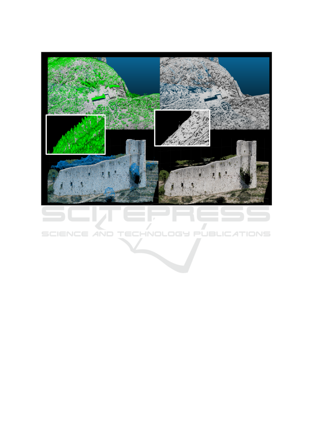
Figure 3: Input data: Oberjettenberg (top) and Gubbio (bottom). In the middle, a detailed view on the rock is shown (Oberjet-
tenberg). The vegetation points are denoted in green (top left) and blue color (bottom left) and removed in the right images.
terns, occlusions, and weak textures. The positive as-
pect, which we intend to exploit, is that RGB values
are available for points together with their XYZ coor-
dinates, as Fig. 2, bottom, shows.
4.2 Ground Surface Filtering
We start by presenting qualitative results for the al-
gorithm based on superpoints. In Fig. 3, we can see
the visually successful filtering result. Most trees and
bushes visible on the left have been filtered out while
the density of points in non-vegetation regions re-
mains approximately the same. In the middle frag-
ment, it seems that from the abundant forest on the
mountain slope, only one single tree trunk remains.
What happens with a small alpine hut in the top im-
age is certainly worth discussion: the lower parts of
it (those which have contact with the ground) remain
while the higher parts have been filtered away: In our
model assumption, there are no other points as terrain
or vegetation. In the Gubbio dataset, it is clear that
some tufts of grass on the wall remain since intensity
was not used for filtering.
For quantitative results, we had to cope with the
fact that both datasets, Oberjettenberg and Gubbio,
are lacking the ground truth. One obvious strategy,
which is chosen in the scope of this work, is to select
a fragment of the data, consisting of some 325 and
500 thousands points, and to create the ground truth
by ourselves, using a (couple of) very salient char-
acteristics of the point cloud followed by an exten-
sive manual relabeling. In order to avoid correlation-
based falsification of results, these salient character-
istics should ideally not have much in common with
our methodology based on superpoints. Thus, we re-
lied on dataset-specific features presented at the end
of Section 3.4: Distance to the DTM (Bulatov et al.,
2012) for the first dataset and spectral indices of RGB
values of 3D points were thus selected.
Tables 1 and 2 reveal that the proposed method
allows to obtain good, plausible, and well-balanced
results. In particular, for the Oberjettenberg dataset,
the accuracy is quite high because a lion’s share of
points belong to the class terrain. As a source for er-
rors, we identified trenches: these are points lying be-
low the plane proposed by RANSAC. In the Gubbio
dataset, porosity and erosion of the wall rock, being
two important aspects why the whole project was in-
stituted, is one of reasons why the algorithm struggles
in its performance. The most important reason, how-
ever, are biases the point cloud itself brings about: as
a result of the photogrammetric procedure for dense
Superpoints in RANSAC Planes: A New Approach for Ground Surface Extraction Exemplified on Point Classification and Context-aware
Reconstruction
31

Table 1: Quantitative results of SIRP for the Oberjettenberg
dataset. Bottom right entry: Overall accuracy (in %). Right
column and bottom row: percentages for precision and re-
call; other entries correspond to the numbers of points. Ter.
= terrain.
True/pred Ter. Non-ter. Total Prec.
Ter. 265867 124 265991 100.0
Non-ter. 4112 55033 59145 93.0
Total 269979 55157 325136 -
Recall 98.5 99.8 - 98.7
Table 2: Quantitative results of SIRP for the Gubbio dataset.
Please refer to Table 1 for additional explanations.
True/pred Ter. Non-ter. Total Prec.
Ter. 131714 7711 139425 94.5
Non-ter. 106091 245768 351859 69.8
Total 237805 253479 491284 -
Recall 55.4 97.0 - 76.9
reconstruction, tree crowns tend to be approximated
by a smooth surface, similar to ground and wall.
4.3 Point Classification
The point sets selected for evaluation in the previ-
ous section were subdivided to nearly equal parts into
training and validation set. The training data was bal-
anced to a relationship not exceeding 2:1. For quali-
tative evaluation, we colored the points of any of the
four categories by a separate color in Fig. 4. For the
Oberjettenberg dataset, we see that, despite of over-
all plausible results, covariance-based classification
leads to more points along the mountain slope that
were spuriously classified as vegetation. For FPFHs,
points atop of the trees are sometimes assigned to
a wrong class. Fortunately, the wrongly classified
points lie mostly isolated, and thus one can expect that
using neighborhood relations (MRFs), we can easily
correct their labels. Different is the situation for the
Gubbio dataset, where the wrongly classified points
build clusters. They are visible on the margin of the
dataset as well as in the regions bordering classes.
But also here, it is clearly visible that FPFHs perform
much better than covariance-based features.
As for quantitative evaluation, we derived the
numbers of true/false positives/negatives and, consis-
tently, the usual metrics like precision, recall, and
overall accuracy. It could be confirmed that the Gub-
bio dataset is much more complicated than the Ober-
jettenberg dataset. While for the latter, the most fa-
vorable parameters of FPFH features yield an over-
all accuracy of 94.6%, it was only around 81.5% for
the former. Analogously, for covariance-based fea-
tures, the difference between some 93% and 77.2% is
considerable as well. With respect to parameter set-
tings of single sets of the features, most of the find-
ings of (Weinmann, 2016) and (Rusu et al., 2009)
are confirmed. kNN with larger neighborhoods usu-
ally performs slightly faster than using radius search
and the quantitative results are comparable; only in
the qualitative results, misclassifications tend to lie
more in clusters and are therefore better visible. In-
teresting is the combination of covariance-based and
FPFH-based features. The results become more sta-
ble (around 95% overall accuracy for Oberjettenberg
and 82% for Gubbio), even though the combination
covariance-based + kNN + small neighborhoods is
non-conductive for the Gubbio dataset. As for includ-
ing dataset-specific features into the configurations,
they helped creating the ground truth and are there-
fore biased. Already local results exhibit a value of
overall accuracy exceeding 95% and thus we exclude
these configurations from the subsequent analysis of
non-local optimization with MRFs.
Considering the quantitative results for MRFs, we
decided to seek answers for two questions: First,
for the parameter set leading to the so far best lo-
cal result (FPFH features with kNNs and 500 neigh-
bors), how much performance improvement can still
be achieved? Second, for a configuration leading to
a fair result (covariance-based features), to what ex-
tent MRFs can help to improve it? In Fig. 5, we note
a somehow similar performance for both datasets and
configurations. The overall accuracy increases until a
certain point and then it decreases or stagnates with
some fluctuations caused, probably, by randomness
of methods and inaccuracies of training data. The de-
crease is even much more visible and significant if the
overall accuracy is replaced by the Cohen κ coeffi-
cient, which considers the fact that the classes are not
necessarily well-balanced. Even though the curves do
not differ strongly in their courses, we can see that
the results for the Oberjettenberg dataset remain bet-
ter for all values of λ than for the Gubbio dataset.
More specifically, for the Gubbio dataset, covariance-
based features are not sufficient, and even the best im-
provement with MRFs does not reach the quality of
the local result with FPFHs, but is approximately 5%
lower. For the Oberjettenberg dataset, however, ap-
plying MRFs to the covariance-based features, which
are simpler as well as easier to compute and to in-
terpret than FPFHs, leads to almost the same result
even though that of local configuration is four per-
cent points below. Thus, a good performance of the
tried-and-true MRFs with a negligible runtime and
with quite a few parameters to determine (λ and N ) is
an encouraging fact. Two reasons why the improve-
ment of the FPFH result is not that significant are:
the point neighborhoods are already extensively taken
GRAPP 2020 - 15th International Conference on Computer Graphics Theory and Applications
32
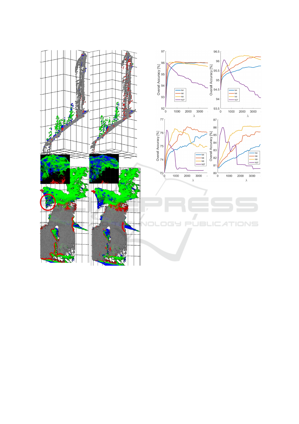
Figure 4: Qualitative classification results for fragments of
datasets Oberjettenberg (top row) and Gubbio (bottom row)
using FPFHs and covariance-based features (left and right
images, respectively). By gray and green points, we de-
noted the correctly classified parts of the terrain (wall in the
case of Gubbio) and vegetation. Blue are points spuriously
classified as terrain and red as vegetation. Middle: a more
detailed view of the tree crown over the Gubbio city wall
(as indicated by the red circumference).
into account and the smoothness prior is less sophis-
ticated. Analogously, if more neighbors (N from (6))
are taken into account, the decay will be faster, as the
violet curves in all images show.
Figure 5: Results for MRF-based classification (Oberjetten-
berg (top) and Gubbio (bottom)) for different feature sets
(left: covariance-based features, right: FPFHs), and differ-
ent neighborhood sizes (colors of the curves with N denot-
ing the number of neighbors). In all curves, overall accuracy
as a function of smoothness parameter λ is shown.
4.4 Application: Surface
Reconstruction
As a possible application, we considered surface re-
construction from points by means of the state-of-the-
art procedure (Kazhdan et al., 2006) and representa-
tion of the surface in different spectral ranges. In the
visualization of Fig. 6, the overhang looks impres-
sively and the 3D character of the point cloud is obvi-
ous. Using an advanced renderer (Feldmann, 2015),
bottom, we believe that the goal of photo-realistic rep-
resentation of this part of the data was achieved. Once
vegetation points have been filtered out, computation
of oriented normal vector field and iso-surface extrac-
tion are relatively robust. The size of the cleaned
point cloud yields 4.4 millions faces while the original
mesh has 5.5 millions faces (almost 26% more) and it
is clear from Fig. 6 that, if we compress point clouds
by means of a mesh decimation algorithm, the image
on the right will be by far more appealing and accu-
rate than that on the left, because it is smoother and
no faces connecting different trees will be built. For
Gubbio (compression factor 30%), the cleaned point
cloud probably looks less appealing than the colored
Superpoints in RANSAC Planes: A New Approach for Ground Surface Extraction Exemplified on Point Classification and Context-aware
Reconstruction
33

one in Fig. 2, bottom. However, this has probably less
to do with aforementioned problems than with the fact
that texturing was not in the scope of this work.
4.5 Computing Times
The method for superpoint-based ground surface fil-
tering is able to process some 6700/7800 points or,
alternatively, 450/53 superpoints (in case of Oberjet-
tenberg/Gubbio) per second. For this, a MATLAB
implementation on a server was used, whereby some
acceleration took place for RANSAC (as described in
Section 3.2). Surprisingly, this was almost that fast
than for 5-core FPFHs using a C++ implementation
in the Point Cloud Library employed for feature com-
putation, for which we recorded some 8200 points/s
and which allowed feature collection in less than one
minute for the test point cloud consisting of almost
500,000 points. We can conclude that a single core
implementation would need some 5 minutes. Other
feature sets are more computationally expensive: For
PFHs, the computation time explodes quadratically
with the neighborhood size while the performance
was roughly the same (factor 36 for kNN of a neigh-
borhood size of 150). Even the covariance-based fea-
tures needed longer using a single-core neighborhood
computation (factor of speed 0.47 for small and 1.4
for large neighborhoods). Classification (tree bag-
ging) and non-local optimization (on MRFs) require
negligible time. Bearing the application of surface re-
construction in mind, the pipeline including ground
surface extraction using our method and point classi-
fication using multi-core FPFHs needs negligible time
in comparison with Poisson reconstruction (Kazhdan
et al., 2006) and should therefore be carried out in
order to guarantee an acceptable input for this com-
putationally expensive method.
4.6 Concluding Remarks on
Comparison with Other Approaches
One should always be cautious while comparing the
results of different approaches applied to different
datasets, because one is always a bit more difficult
than another. Even within our datasets, we cannot
completely be sure that the manually created ground
truth is good enough. Assuming that there are few
errors in the reference, the most interesting insight
of our work is that, at least for the LiDAR dataset,
the proposed method, which does not need any train-
ing points, outperforms the rotation-invariant feature
sets used for supervised classification. Taking into ac-
count quite comparable computation times, the bene-
fit of SIRP is evident. For the second dataset, its per-
formance is slightly worse than that of FPFHs (76.9%
in Table 2 vs. 81 to 87 % in Fig. 5, bottom right). At
least, the covariance-based features could be left be-
hind (Fig. 5, bottom left). The fact that SIRP does not
need any training data is beneficial for the alternative
evaluation strategy: To run it – with the same param-
eters – on a less challenging dataset, however, with
labeled ground truth. This strategy is currently being
implemented. Finally, one of the newest approaches
on CNN-based multi-class semantic segmentation on
airborne remote sensing data (Winiwarter et al., 2019)
has produced the results of roughly the same order of
magnitude.
5 DISCUSSION AND OUTLOOK
We start this section with the critical discussion about
the newly presented SIRP method. It basically relies
on the fact that the terrain is locally planar whereby
plane orientation is of secondary importance. The
size of the infinitesimal planar patch is given by the
superpoint while the plane search is accomplished by
a smart, loopless implementation of the RANSAC
procedure. On the one hand, generalizing this method
for second degree surfaces (conics) – in order to deal
with abrupt changes of terrain curvature and model-
ing tree shapes – would represent a mathematical-
theoretical challenge. On the other hand, RANSAC
already occupies the major resources of the comput-
ing time of SIRP even though, in the future, it can
be parallelized. Concerning the performance, we ob-
served a quite high overall accuracy given that we in-
tentionally worked with 3D information and did not
use intensity or knowledge about the z axis: SIRP is
widely rotation-invariant. We could say that SIRP,
in combination with other source- or application-
dependent features is a very suitable tool for extrac-
tion of ground truth. For a photogrammetric dataset,
RGB colors may provide a great alleviation. For the
Oberjettenberg dataset, where we already mentioned
the problem of trenches, one could allow more tol-
erance into the direction of superpoint interior. How-
ever, our RANSAC planes are not oriented and impos-
ing consistent orientation is a non-trivial task (Hoppe
et al., 1992). The clustering step is particularly help-
ful because it allows cutting away (possibly) large
parts of data assigned to a wrong class using an in-
teractive tool, such as Cloud Compare
3
.
Coming to the features, we could see that applica-
tion of covariance-based features, Fast Point Feature
Histograms, and Markov Random Fields is reason-
3
https://www.danielgm.net/cc/
GRAPP 2020 - 15th International Conference on Computer Graphics Theory and Applications
34
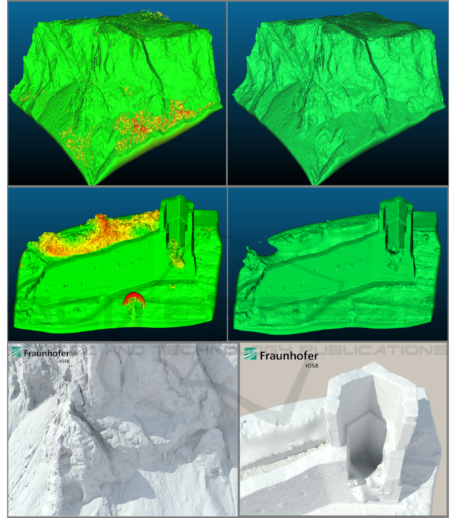
Figure 6: Surface reconstruction results from the original point cloud (left) and from the cleaned point cloud (right) for the
Oberjettenberg dataset (part of the data, top) and for the Gubbio dataset (middle). The mesh on the left is colored according to
the vertical distance to the mesh on the right, truncated by the maximum value of 30 m. Bottom: fragments of photo-realistic
representations of Oberjettenberg and Gubbio datasets (left and right, respectively) using a path-tracer (Feldmann, 2015),
(courtesy of Eva Burkard).
able, however, the impacts are different. Covariance-
based features are easier to interpret and to compute,
but FPFHs are faster and better. It is worth men-
tioning that, after post-processing, the performance of
covariance-based features is quite comparable to that
of FPFHs in the case of laser point clouds. For pho-
togrammetric point clouds, there is still a gap in the
performance. Also, we saw that for a high number
Superpoints in RANSAC Planes: A New Approach for Ground Surface Extraction Exemplified on Point Classification and Context-aware
Reconstruction
35

of neighbors, MRFs have not contributed to an im-
provement. Here, their replacement with Conditional
Random Fields, which additionally take into account
the strength of inferences, may help. Finally, it must
be mentioned that feature sets and MRFs are appli-
cable to multi-class problems as well. Testing their
performance is clearly a subject of our future work.
ACKNOWLEDGEMENTS
We wish to thank all those people who made avail-
able for public the software for: (F)PFH (Point Cloud
Library), Graph Cuts on MRFs (Delong et al., 2012),
and interactive point clouds processing (Cloud Com-
pare). We also thank Ms. Eva Burkard (IOSB) for
visualizing the 3D meshes in the path-tracer.
REFERENCES
Boykov, Y., Veksler, O., and Zabih, R. (2001). Fast ap-
proximate energy minimization via graph cuts. IEEE
Transactions on Pattern Analysis and Machine Intel-
ligence, 23(11):1222–1239.
Breiman, L. (2001). Random forests. Machine Learning,
45(1):5–32.
Bulatov, D., Lucks, L., Moßgraber, J., Pohl, M., Solbrig,
P., Murchio, G., and Padeletti, G. (2018). HERA-
CLES: EU-backed multinational project on cultural
heritage preservation. In Earth Resources and Envi-
ronmental Remote Sensing/GIS Applications IX, vol-
ume 10790, pages 78–87. International Society for
Optics and Photonics.
Bulatov, D., Wernerus, P., and Gross, H. (2012). On ap-
plications of sequential multi-view dense reconstruc-
tion from aerial images. In Proceedings of the Inter-
national Conference on Pattern Recognition Applica-
tions and Methods, pages 275–280.
Carvalho, F., Lopes, A., Curulli, A., da Silva, T., Lima, M.,
Montesperelli, G., Ronca, S., Padeletti, G., and Veiga,
J. (2018). The case study of the medieval town walls
of Gubbio in Italy: first results on the characterization
of mortars and binders. Heritage, 1(2):468–478.
Delong, A., Osokin, A., Isack, H. N., and Boykov, Y.
(2012). Fast approximate energy minimization with
label costs. International Journal of Computer Vision,
96(1):1–27.
Elmqvist, M., Jungert, E., Lantz, F., Persson, A., and
S
¨
oderman, U. (2001). Terrain modelling and analy-
sis using laser scanner data. International Archives
of the Photogrammetry, Remote Sensing and Spatial
Information Sciences, 34(3/W4):219–226.
Evans, D. H., Fletcher, R. J., Pottier, C., Chevance, J.-B.,
Soutif, D., Tan, B. S., Im, S., Ea, D., Tin, T., Kim, S.,
et al. (2013). Uncovering archaeological landscapes
at angkor using lidar. Proceedings of the National
Academy of Sciences, 110(31):12595–12600.
Feldmann, D. (2015). Accelerated ray tracing using R-
trees. In International Joint Conference on Computer
Vision, Imaging and Computer Graphics Theory and
Applications, pages 247–257. INSTICC.
Fischler, M. A. and Bolles, R. C. (1981). Random sample
consensus: A paradigm for model fitting with appli-
cations to image analysis and automated cartography.
Commun. ACM, 24(6):381–395.
Gross, H. and Thoennessen, U. (2006). Extraction of lines
from laser point clouds. International Archives of the
Photogrammetry, Remote Sensing and Spatial Infor-
mation Sciences, 36(3):86–91.
Guo, X., Xiao, J., and Wang, Y. (2018). A survey on al-
gorithms of hole filling in 3D surface reconstruction.
The Visual Computer, 34(1):93–103.
Hackel, T., Wegner, J. D., and Schindler, K. (2016). Fast se-
mantic segmentation of 3D point clouds with strongly
varying density. ISPRS Annals of the Photogramme-
try, Remote Sensing and Spatial Information Sciences,
3(3):177–184.
Hana, X.-F., Jin, J. S., Xie, J., Wang, M.-J., and Jiang, W.
(2018). A comprehensive review of 3d point cloud
descriptors. arXiv preprint arXiv:1802.02297.
H
¨
aufel, G., Bulatov, D., and Solbrig, P. (2017). Sensor data
fusion for textured reconstruction and virtual repre-
sentation of alpine scenes. In Earth Resources and
Environmental Remote Sensing/GIS Applications VIII,
volume 10428, pages 33–46.
Hoppe, H., DeRose, T., Duchamp, T., McDonald, J., and
Stuetzle, W. (1992). Surface reconstruction from un-
organized points. ACM SIGGRAPH Computer Graph-
ics, 26(2):71–78.
Kazhdan, M., Bolitho, M., and Hoppe, H. (2006). Poisson
surface reconstruction. In Proceedings of the Fourth
Eurographics Symposium on Geometry Processing,
pages 61–70.
Kraus, K. and Pfeifer, N. (1998). Determination of terrain
models in wooded areas with airborne laser scanner
data. ISPRS Journal of Photogrammetry and Remote
Sensing, 53(4):193–203.
Lafarge, F. and Mallet, C. (2012). Creating large-scale city
models from 3D-point clouds: a robust approach with
hybrid representation. International Journal of Com-
puter Vision, 99(1):69–85.
Lalonde, J.-F., Unnikrishnan, R., Vandapel, N., and Hebert,
M. (2005). Scale selection for classification of point-
sampled 3D surfaces. In Proceedings of the Fifth In-
ternational Conference on 3-D Digital Imaging and
Modeling (3DIM’05), pages 285–292. IEEE.
Mongus, D. and
ˇ
Zalik, B. (2012). Parameter-free ground
filtering of LiDAR data for automatic DTM genera-
tion. ISPRS Journal of Photogrammetry and Remote
Sensing, 67:1–12.
Mousa, Y. A., Helmholz, P., Belton, D., and Bulatov, D.
(2019). Building detection and regularisation using
DSM and imagery information. The Photogrammetric
Record, 34(165):85–107.
Perko, R., Raggam, H., Gutjahr, K., and Schardt, M. (2015).
Advanced DTM generation from very high resolution
GRAPP 2020 - 15th International Conference on Computer Graphics Theory and Applications
36

satellite stereo images. ISPRS Annals of the Pho-
togrammetry, Remote Sensing and Spatial Informa-
tion Sciences, 2(3/W4):165–172.
Qi, C. R., Yi, L., Su, H., and Guibas, L. J. (2017). Point-
Net++: Deep hierarchical feature learning on point
sets in a metric space. In Advances in Neural Infor-
mation Processing Systems, pages 5099–5108.
Raguram, R., Frahm, J.-M., and Pollefeys, M. (2008). A
comparative analysis of RANSAC techniques lead-
ing to adaptive real-time random sample consensus.
In Proceedings of the European Conference on Com-
puter Vision, pages 500–513. Springer.
Rusu, R. B., Blodow, N., and Beetz, M. (2009). Fast point
feature histograms (FPFH) for 3D registration. In
Proceedings of the 2009 IEEE International Confer-
ence on Robotics and Automation, pages 3212–3217.
IEEE.
Rusu, R. B., Marton, Z. C., Blodow, N., and Beetz, M.
(2008). Persistent point feature histograms for 3D
point clouds. In Proceedings of the 10th International
Conference on Intelligent Autonomous Systems, pages
119–128.
Von Hansen, W. (2006). Robust automatic marker-free
registration of terrestrial scan data. International
Archives of the Photogrammetry, Remote Sensing and
Spatial Information Sciences, 36(3):105–110.
Vosselman, G. (2000). Slope based filtering of laser altime-
try data. International Archives of Photogrammetry
and Remote Sensing, 33(B3):935–942.
Weinmann, M. (2016). Reconstruction and Analysis of 3D
Scenes: From Irregularly Distributed 3D Points to
Object Classes. Springer International Publishing, 1st
edition.
Weinmann, M., Jutzi, B., Mallet, C., and Weinmann, M.
(2017). Geometric features and their relevance for
3D point cloud classification. ISPRS Annals of the
Photogrammetry, Remote Sensing and Spatial Infor-
mation Sciences, 4(1/W1):157–164.
Weinmann, M. and Weinmann, M. (2018). Geospatial com-
puter vision based on multi-modal data – how valuable
is shape information for the extraction of semantic in-
formation? Remote Sensing, 10(1):2:1–2:20.
West, K. F., Webb, B. N., Lersch, J. R., Pothier, S., Triscari,
J. M., and Iverson, A. E. (2004). Context-driven auto-
mated target detection in 3D data. In Automatic Target
Recognition XIV, volume 5426, pages 133–144. Inter-
national Society for Optics and Photonics.
Winiwarter, L., Mandlburger, G., Pfeifer, N., and S
¨
orgel, U.
(2019). Classification of 3D point clouds using deep
neural networks. In Dreil
¨
andertagung der DGPF, der
OVG und der SGPF, pages 663–674.
Zhang, K., Chen, S.-C., Whitman, D., Shyu, M.-L., Yan,
J., and Zhang, C. (2003). A progressive morphologi-
cal filter for removing nonground measurements from
airborne lidar data. IEEE Transactions on Geoscience
and Remote Sensing, 41(4):872–882.
Superpoints in RANSAC Planes: A New Approach for Ground Surface Extraction Exemplified on Point Classification and Context-aware
Reconstruction
37
